Part 1.1: Convolutions from Scratch
I implemented 2D convolution three ways to understand performance trade-offs:
1.1.1 Three Convolution Implementations
Implementation 1: Naive (4 loops)
Implementation 2: Optimized (2 loops)
Implementation 3: Using SciPy
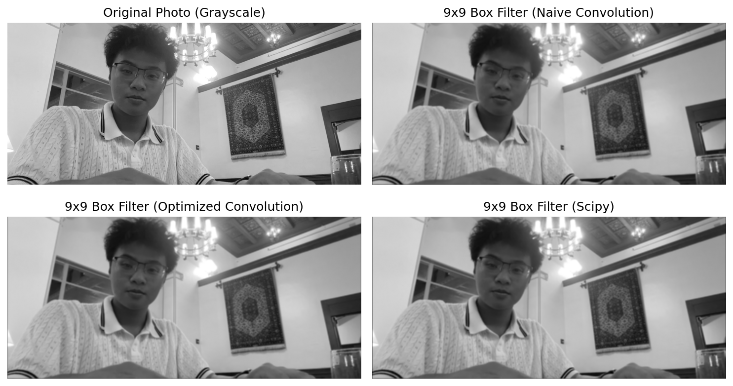
1.1.2 Testing with 9×9 Box Filter
Creating a Box Filter
| Implementation | 9×9 Box Filter | Speedup | Max Error |
|---|---|---|---|
| Naive | 32.65s | 1× | < 10⁻¹⁵ |
| Optimized | 3.03s | 10.8× | |
| Scipy | 0.11s | 295× |
Accuracy Verification
Naive vs Scipy max difference: 2.44 × 10⁻¹⁵
Optimized vs Scipy max difference: 7.77 × 10⁻¹⁶
1.1.3 Finite Difference Operators
Next, I tested with finite difference operators to detect edges:
Finite Difference Operators
| Implementation | Dx Runtime | Dy Runtime |
|---|---|---|
| Naive | 1.47s | 1.60s |
| Optimized | 2.89s | 2.92s |
| Scipy | 0.01s | 0.02s |
Key Observations
• Small kernels (3×3) show naive faster than optimized due to NumPy overhead.
• All implementations produce identical results.
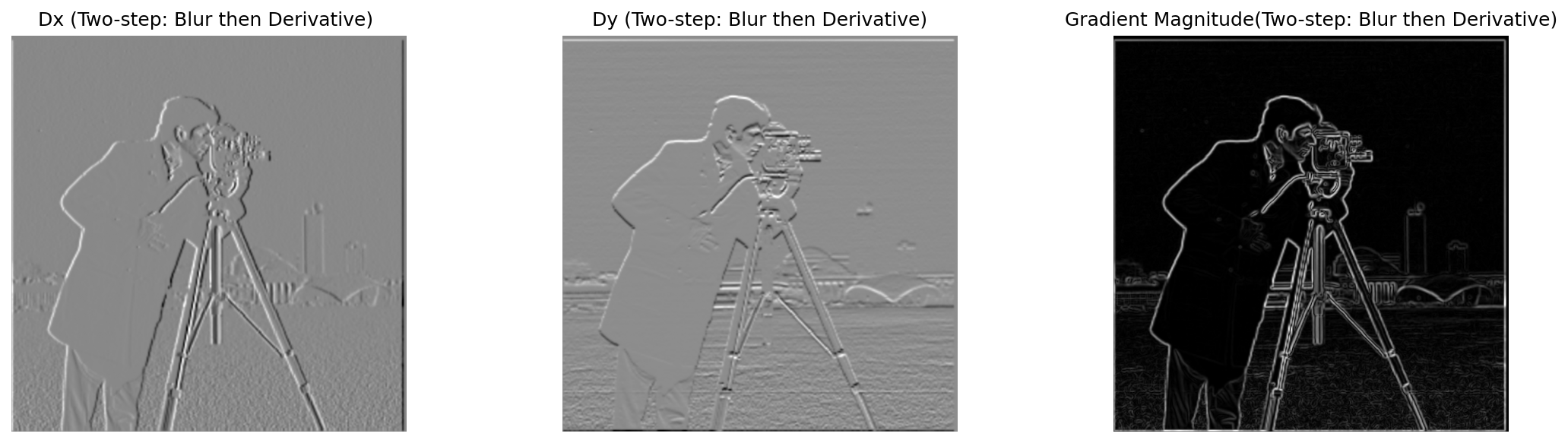
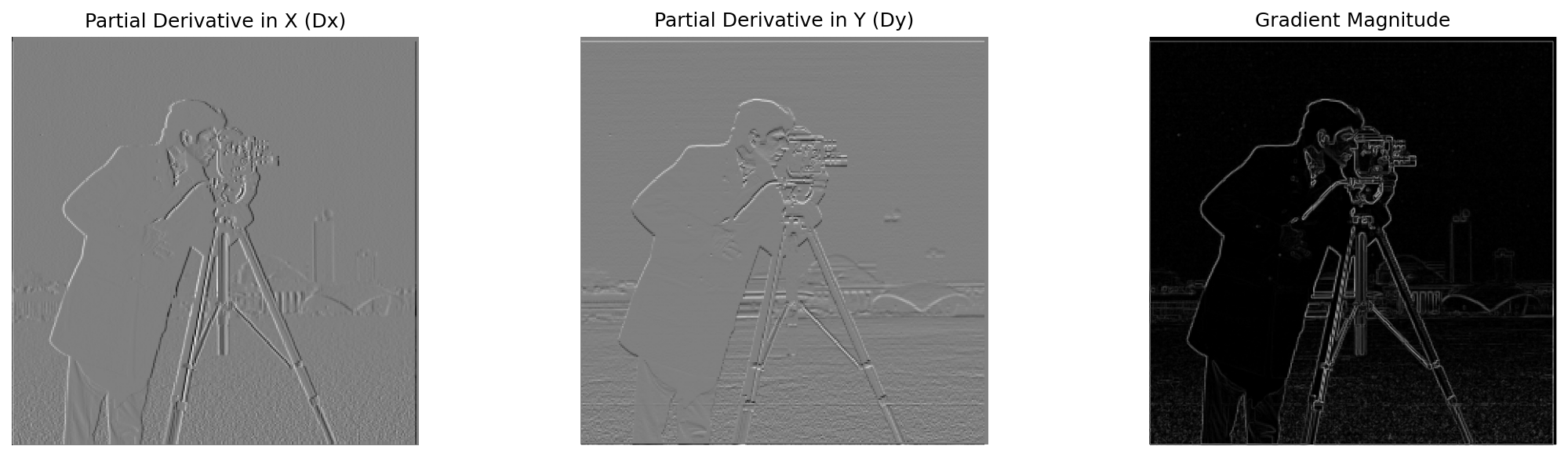
• Dx, Dy outputs: Can be negative or positive, so black = negative, gray = zero, white = positive.
• Gradient Magnitude: Always positive, so black = 0 (no edge), white = strong edge.



Part 1.2: Finite Difference Operator
Edge detection via gradient magnitude and thresholding. After learning how to implement convolution from scratch in Part 1.1, we now use scipy for efficiency.
1.2.1 Applying Finite Difference to Cameraman
Here we apply the same Dx and Dy operators to the classic cameraman.png image and compute the gradient magnitude.
Image Preprocessing
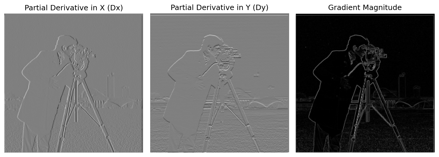
Notice that the contrast is quite poor - the edges appear faint rather than bright white. To address this issue, we need to normalize the gradient magnitude to the range [0,1] and find an optimal threshold to filter out noise -> this is called binary edge detection.
Gradient Normalization
1.2.2 Finding Optimal Threshold
Coarse Search

Fine-tuned Search
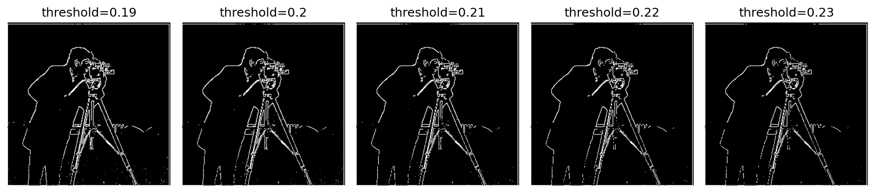
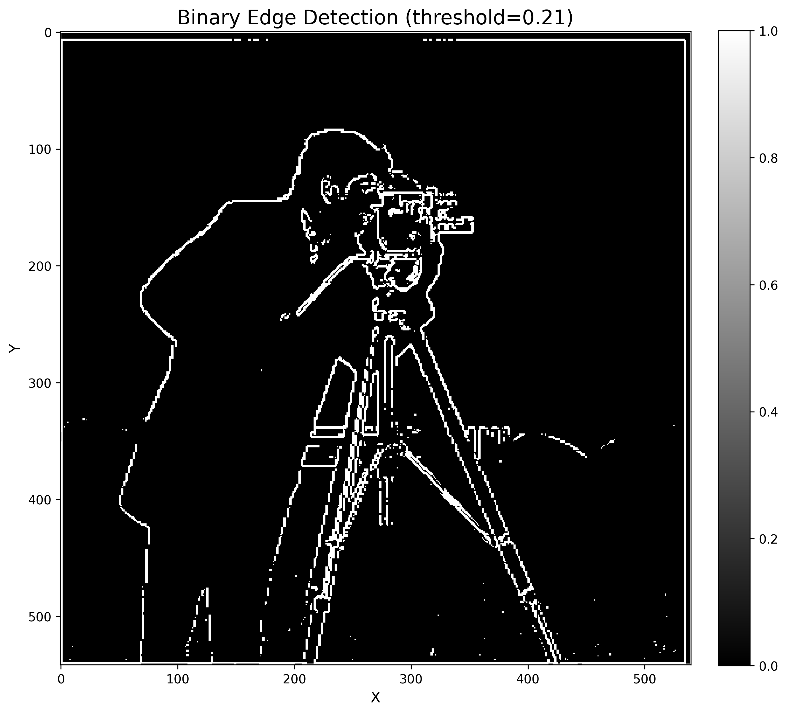
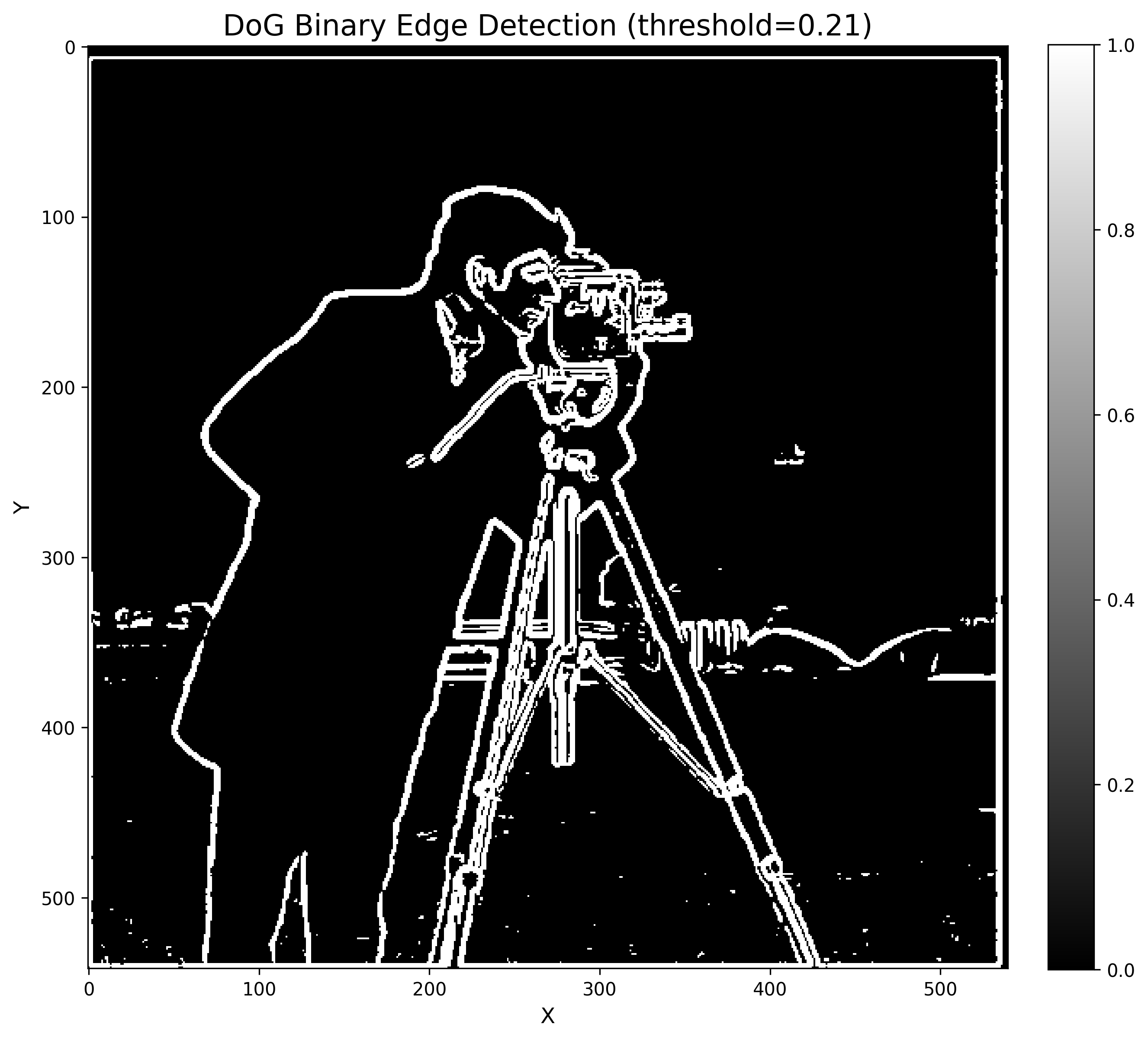
Optimal: T = 0.21
It's a difficult trade-off: if the threshold is higher, it reduces noise but also blurs the real edges of the cameraman.
Since no matter how large the threshold is, the bridge remains as high-frequency as the cameraman, it's impossible to isolate only the cameraman.
Hence, this setting is already the best balance between noise suppression and edge preservation.
Part 1.3: Derivative of Gaussian (DoG) Filter
The edges from Part 1.2 appear noisy. We can improve edge detection by first smoothing the image with a Gaussian filter before computing gradients.
Gaussian Kernel Creation
Understanding σ (Sigma)
σ is the standard deviation that controls the blur intensity:
- Small σ → Sharp, blurs only a small neighborhood
- Large σ → Strong blur, affects a wider range
1.3.1 Two-Step Approach: Blur Then Gradient
First, we apply a Gaussian filter to smooth the image, then compute gradients:
Two-Step Implementation
Why Choose kernel_size=7, sigma=1?
A common choice is to choose k = 6σ + 1
- Gaussian kernel contains most (>99%) of the useful weights
- Kernel size too tiny: cut off the Gaussian
- Kernel size too large: waste compute since outside the ±3σ weights are very close to 0
1.3.2 One-Step Approach: DoG Filters
Due to convolution associativity, we can combine the Gaussian and derivative into a single DoG filter:
DoG Filter Implementation
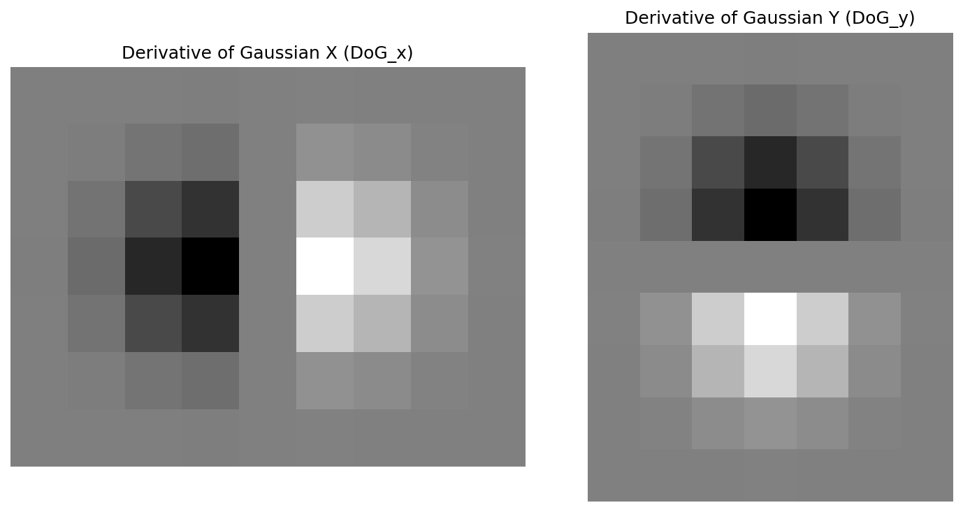
One-Step Implementation: Convolve with DoG
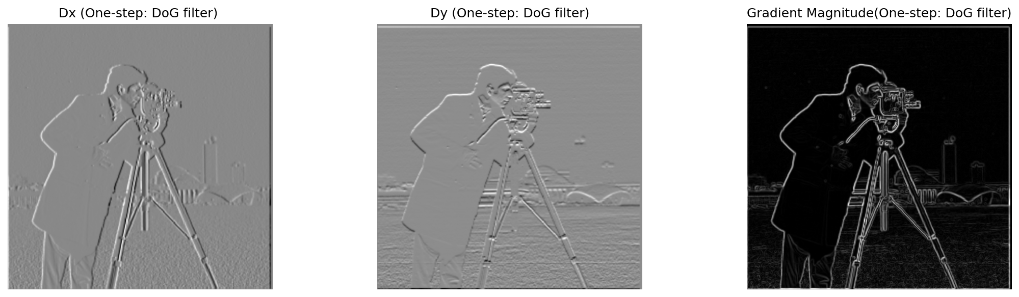
1.3.1 & 1.3.2 Verification: Two-Step vs One-Step
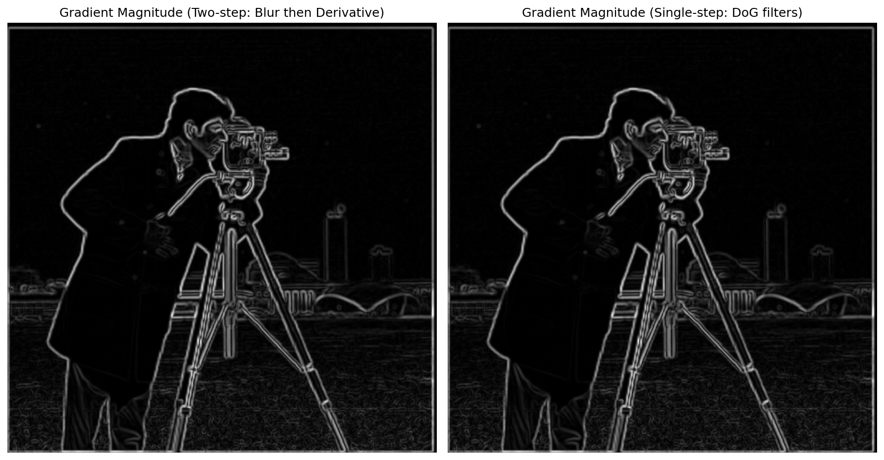
Numerical Verification:
- Max difference in Dx: 0.0000000000
- Max difference in Dy: 0.0000000000
- Max difference in gradient magnitude: 0.0000000000
The results are mathematically identical, confirming the associative property of convolution: (G * I) * D = I * (G * D)
[Note.] Implementation Detail: Convolution Padding
When implementing convolution, using boundary='fill' will produce incorrect results, but boundary='symm' gives the correct output. Here's why:
Why boundary='fill' fails:
- Our kernel size is relatively small (e.g., DoG filter visualization shows edges are still gray, not zero)
- When boundary values are treated as 0 (black), a "dark edge effect" appears at borders
- The convolution kernel near edges mixes in these 0 values → causes brightness reduction and obvious dark frames
Why boundary='symm' (mirror padding) works:
- Boundary values are mirrored symmetrically, like looking in a mirror
- The kernel at edges can still get reasonable values instead of encountering zeros
- The effect is more natural, without dark edges or sudden brightness changes
- Most image processing libraries (OpenCV, Pillow, MATLAB) use mirror/reflection padding by default for sharpening and blurring operations
1.3.3 Comparing Edge Detection: With vs Without Blur
We can find out that with DoG Filter, the edge is clearer since it removes high-frequency noise through Gaussian smoothing while preserving the main edge structures.
(1.2) Without Gaussian Blur
(1.3) With DoG Filter (Gaussian Blur)
1.3.4 Optimal Threshold with DoG
After applying the DoG filter, the high-frequency noise has been removed, which changes the gradient magnitude distribution. Therefore, we need to find a new optimal threshold for edge detection:


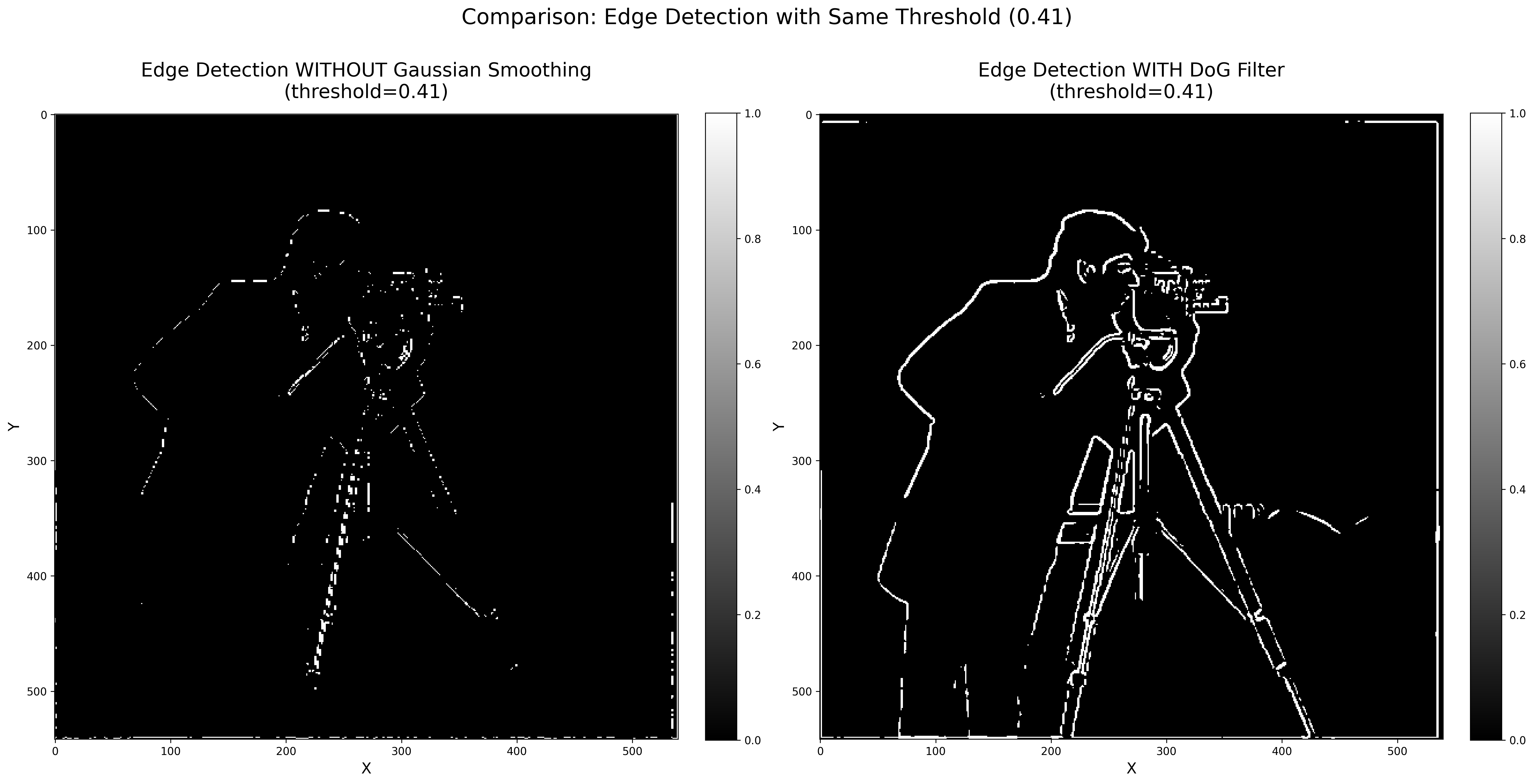
Optimal: T = 0.41
• DoG allows using higher thresholds (0.41 vs 0.21) while preserving important edges
• Without DoG, at threshold 0.41 the edges have already lost half of the details
Part 2.1: Image Sharpening with Unsharp Masking
Unsharp masking sharpens images by first blurring (applying Gaussian filter), then subtracting to get high frequencies (similar to Laplacian), and finally adding them back to enhance edges.
2.1.1 Step-by-Step Implementation
Let's break down the sharpening process into individual steps:
Stepwise Unsharp Masking
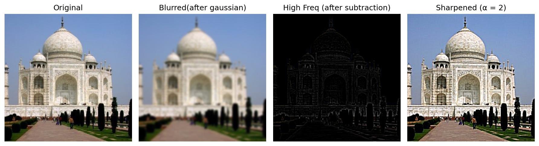
2.1.2 Simplified: Single Unsharp Mask Kernel
We don't need to perform these steps separately. We can combine them into a single unsharp mask kernel and apply it in one convolution:
Unsharp Masking Formula Derivation
= (1 + α) × original - α × blurred
= (1 + α) × original - α × (gaussian ⊗ original)
= [(1 + α) × identity - α × gaussian] ⊗ original
Therefore, the unsharp kernel = (1 + α) × identity - α × gaussian
Where α controls the sharpening strength. Higher α = more pronounced edges.
Note: "identity" here refers to the identity convolution kernel (center=1, rest=0), not the linear algebra identity matrix.
Unsharp Mask Kernel Creation
Convolve with Unsharp Mask Kernel
2.1.3 Testing Different Alpha Values
The α parameter controls sharpening intensity. Let's compare different values:

2.1.4 Blur-Sharpen-Blur-Sharpen Experiment
What happens if we blur a sharpened image and sharpen it again?
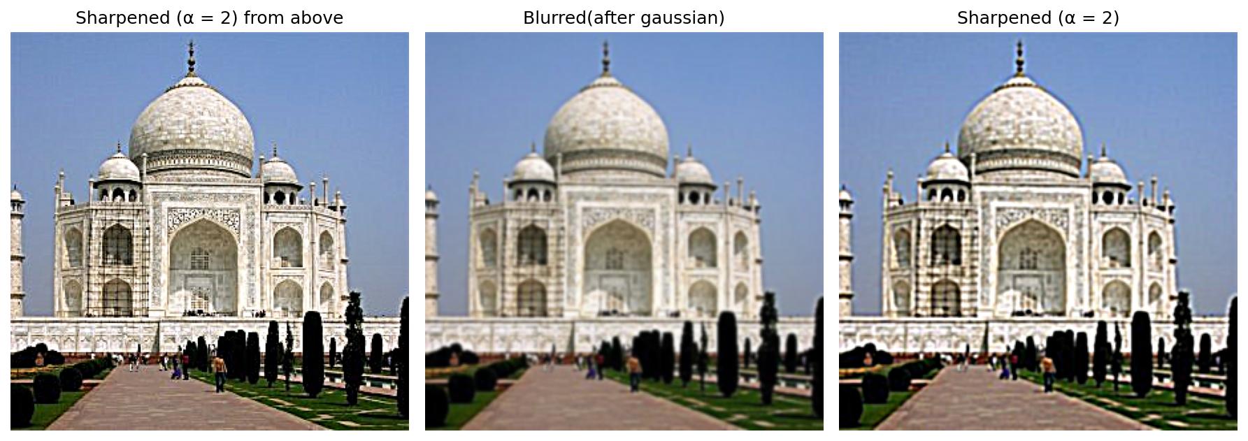
Lesson: Information loss in blurring is irreversible
- Some high-frequency details are permanently lost in the blur step
- The result is softer than the original sharpened version
- We partially recover sharpness, but not fully
2.1.5 Custom Image: Shaved Snow
This image holds special meaning for me — it was taken with friends a week before I came to the US for exchange. The day before taking this photo, I accidentally fell asleep in the bathtub while showering, and my phone got water damaged. Can CS180 techniques rescue this photo?
At first, I loaded the picture as-is, but its shape is (4032, 2268, 3) — way bigger than the Taj image. The default kernel_size=9 is too small to capture many edge details at this resolution. To be honest, I can't really tell the difference:
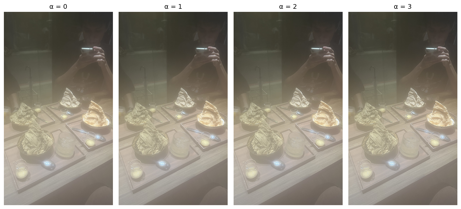
My solution: resize the image using transform.resize(shaved_snow, (600, 337), anti_aliasing=True). Now we can actually see the results:
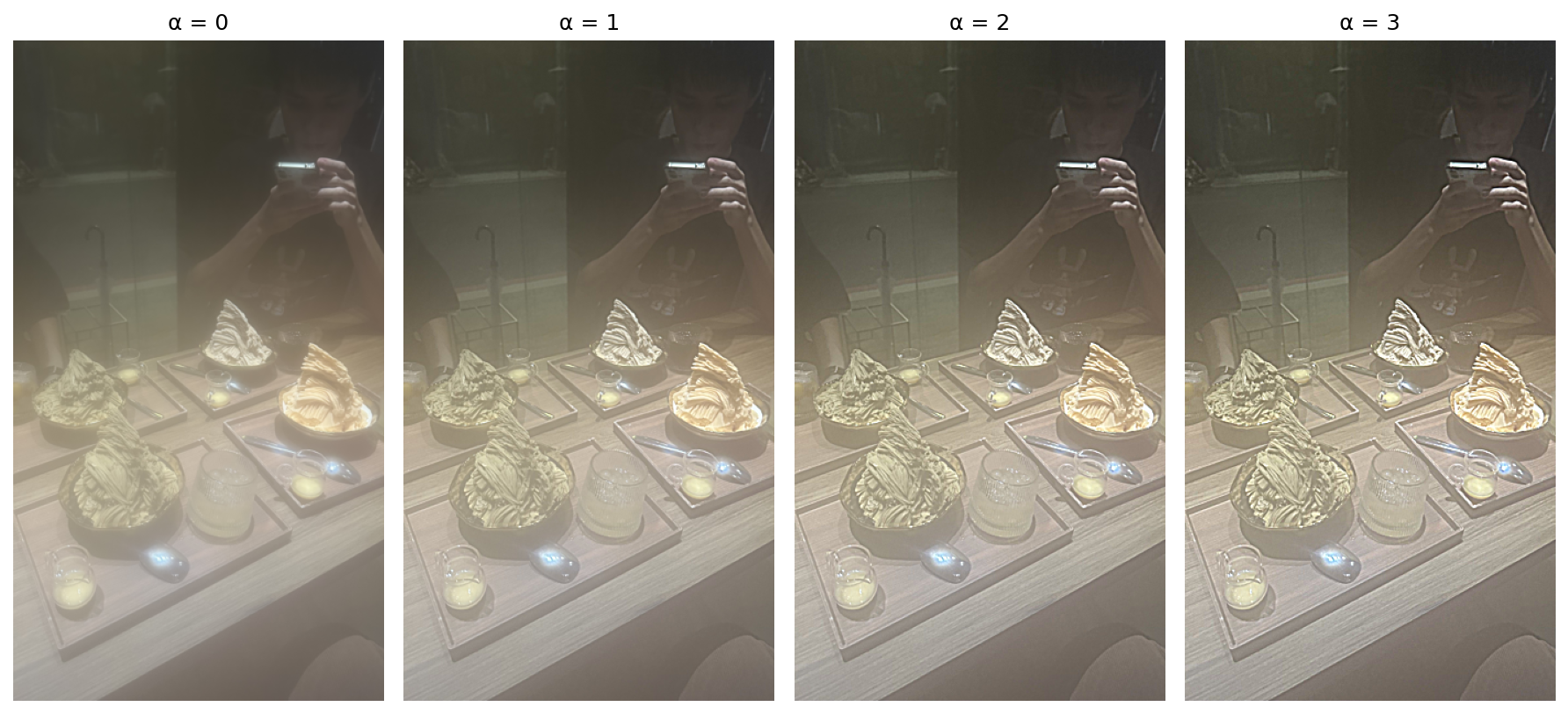
The photo wasn't fully rescued:
- While sharpening helps, it can't fully recover lost details from the water damage.
- No matter how advanced image processing techniques are, the most important thing is still the quality of the original signal
- Kernel size matters: Must be proportional to image resolution for effective sharpening
Part 2.2: Hybrid Images
High-frequency details dominate at close distances, vice versa. By combining the low frequencies of one image with the high frequencies of another, we create an image that changes appearance based on viewing distance.
2.2.1 Image Selection & Originals
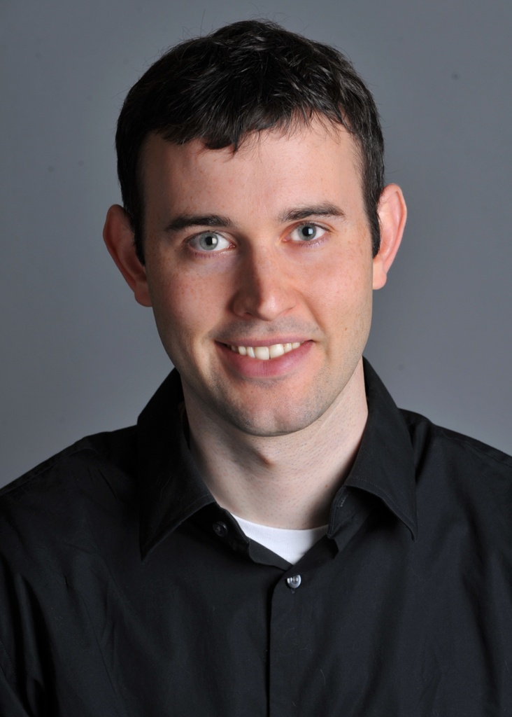
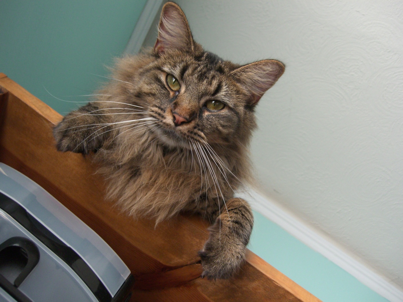
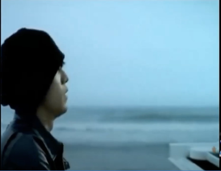
I created three hybrid image pairs. Here are the original photos before alignment and filtering:
Derek + Nutmeg
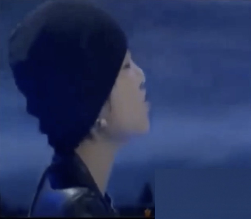
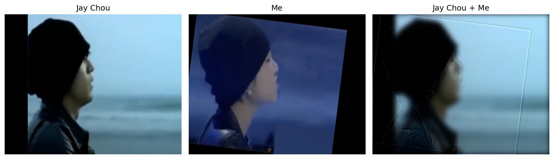
Jay Chou + Me
When I was a child, I appeared on a TV show imitating Asian singer Jay Chou. Now I can see how close the resemblance was!
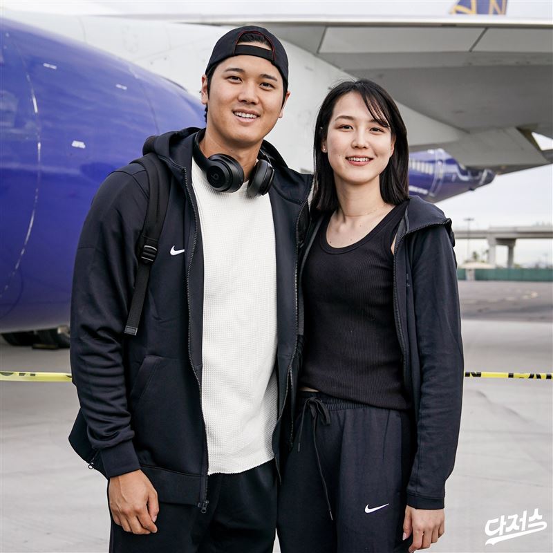
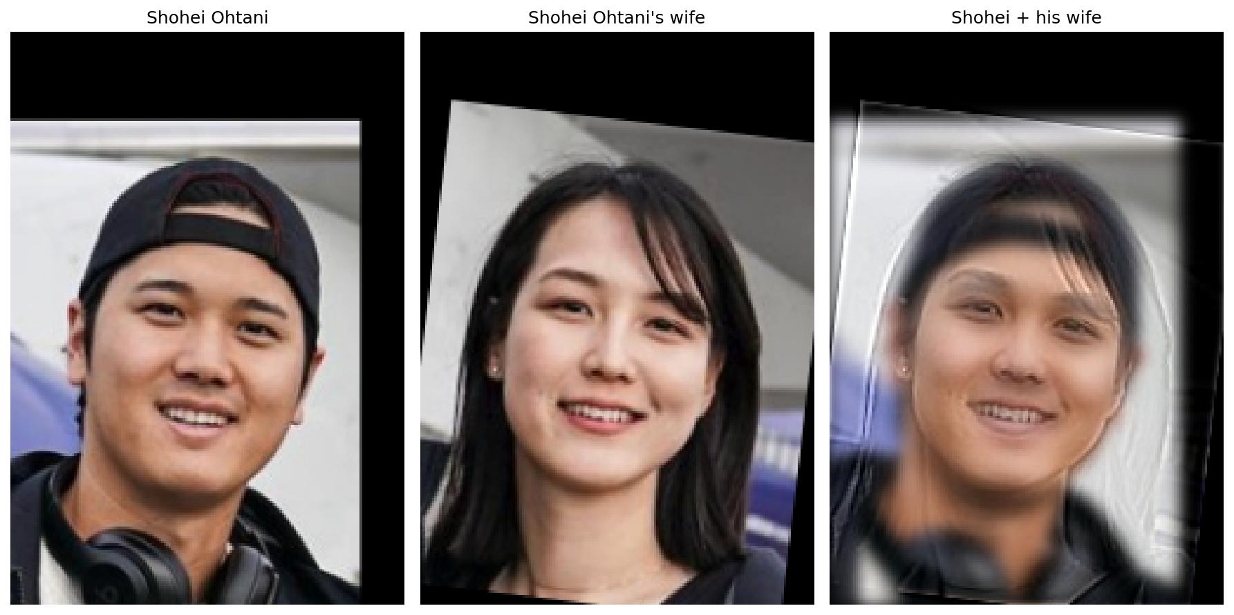
Shohei Ohtani + Wife
I've seen many news articles claiming they have couple faces. Let's see if a hybrid confirms this!
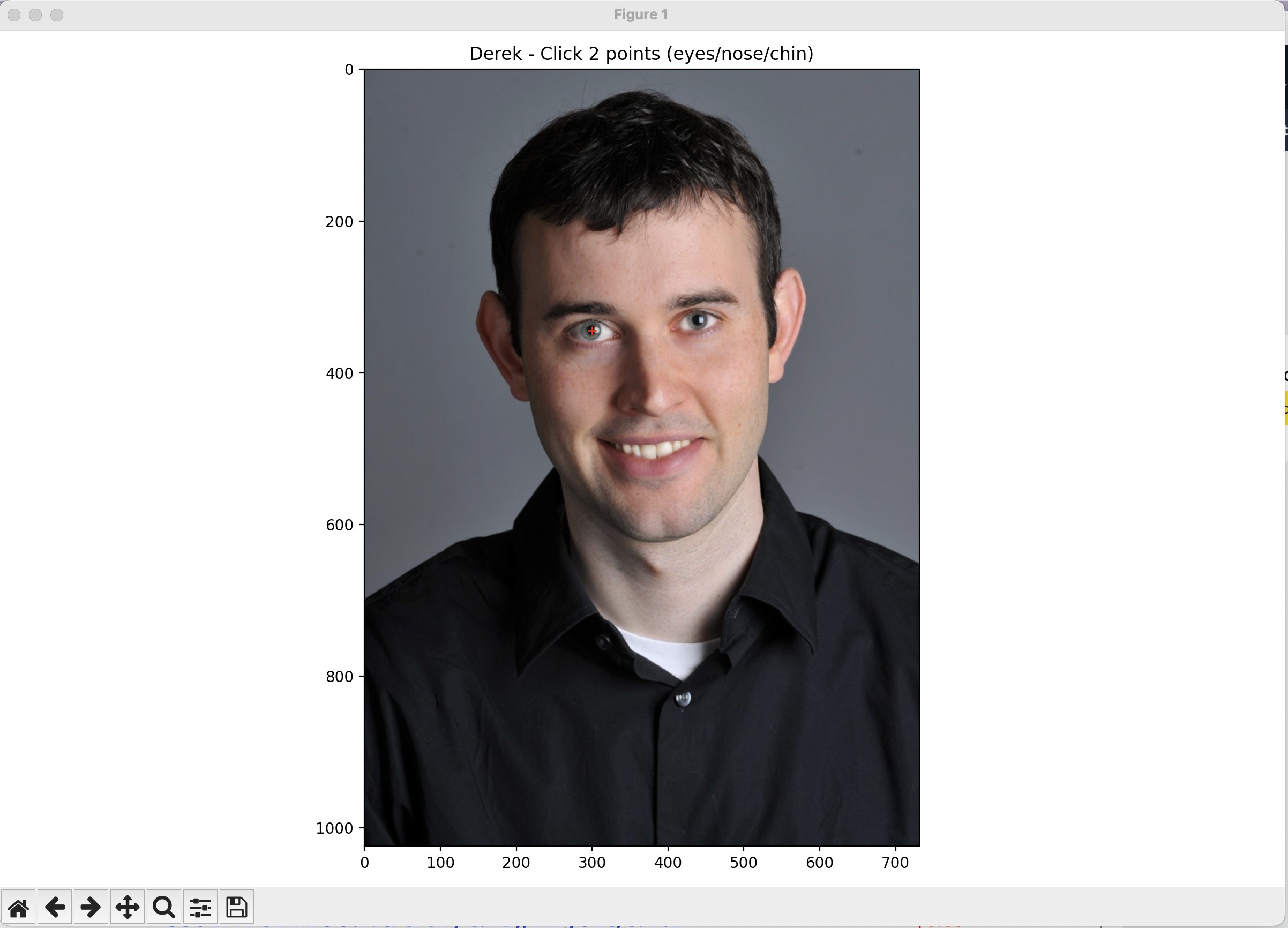
2.2.2 Image Alignment
Before creating hybrid images, we need to align the facial features. I used an interactive clicking tool (part2_2_align_image.py) to manually select two corresponding points on both images, which are then used as anchors for rotation and scaling transformations.
2.2.3 Frequency Filtering Implementation
Low-Pass Filter
High-Pass Filter
Create Hybrid Image
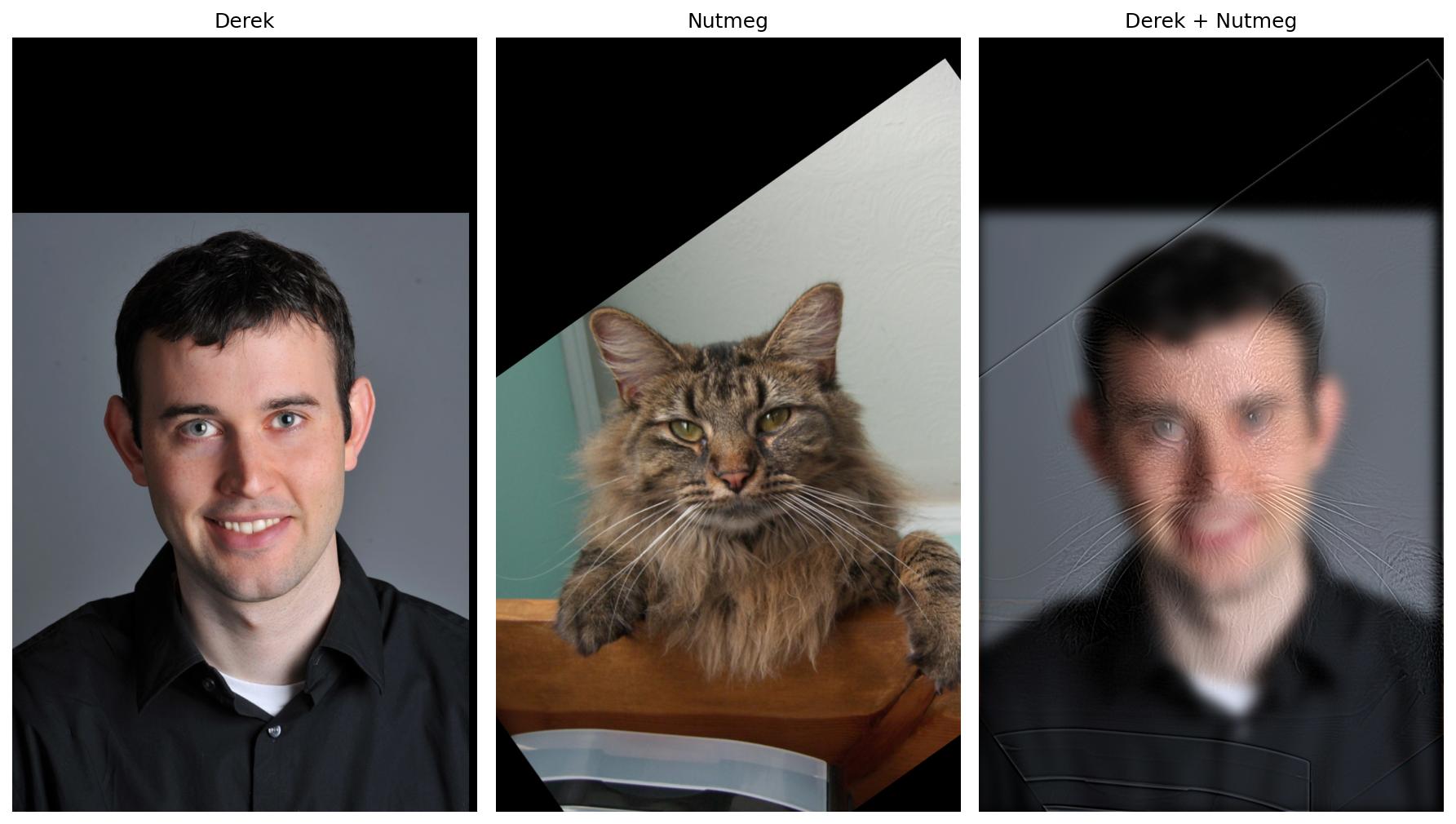
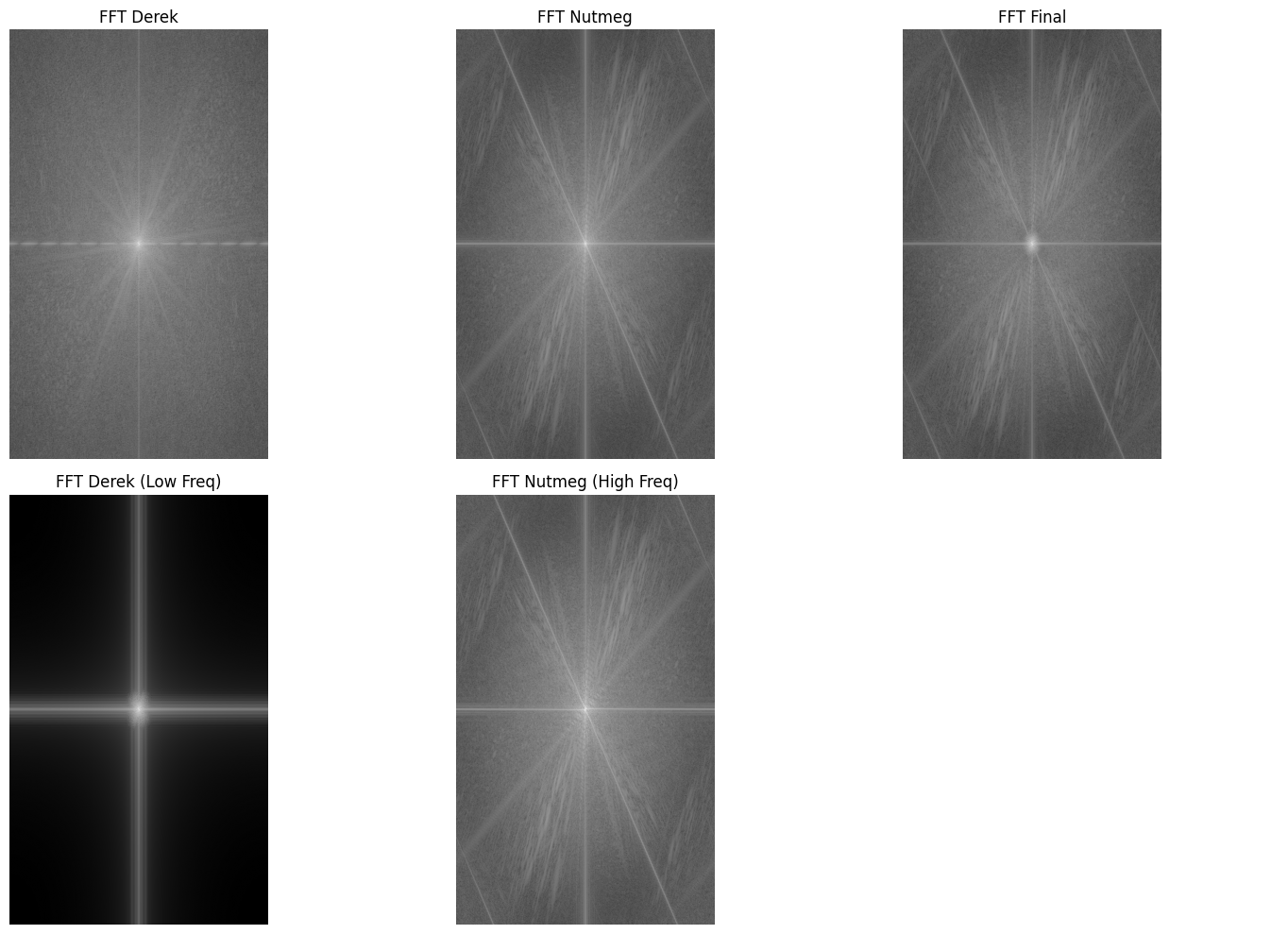
2.2.4 Derek + Nutmeg
Parameters: σlow=10, σhigh=2
2.2.5 Jay Chou + Childhood Me
Parameters: σlow=10, σhigh=3
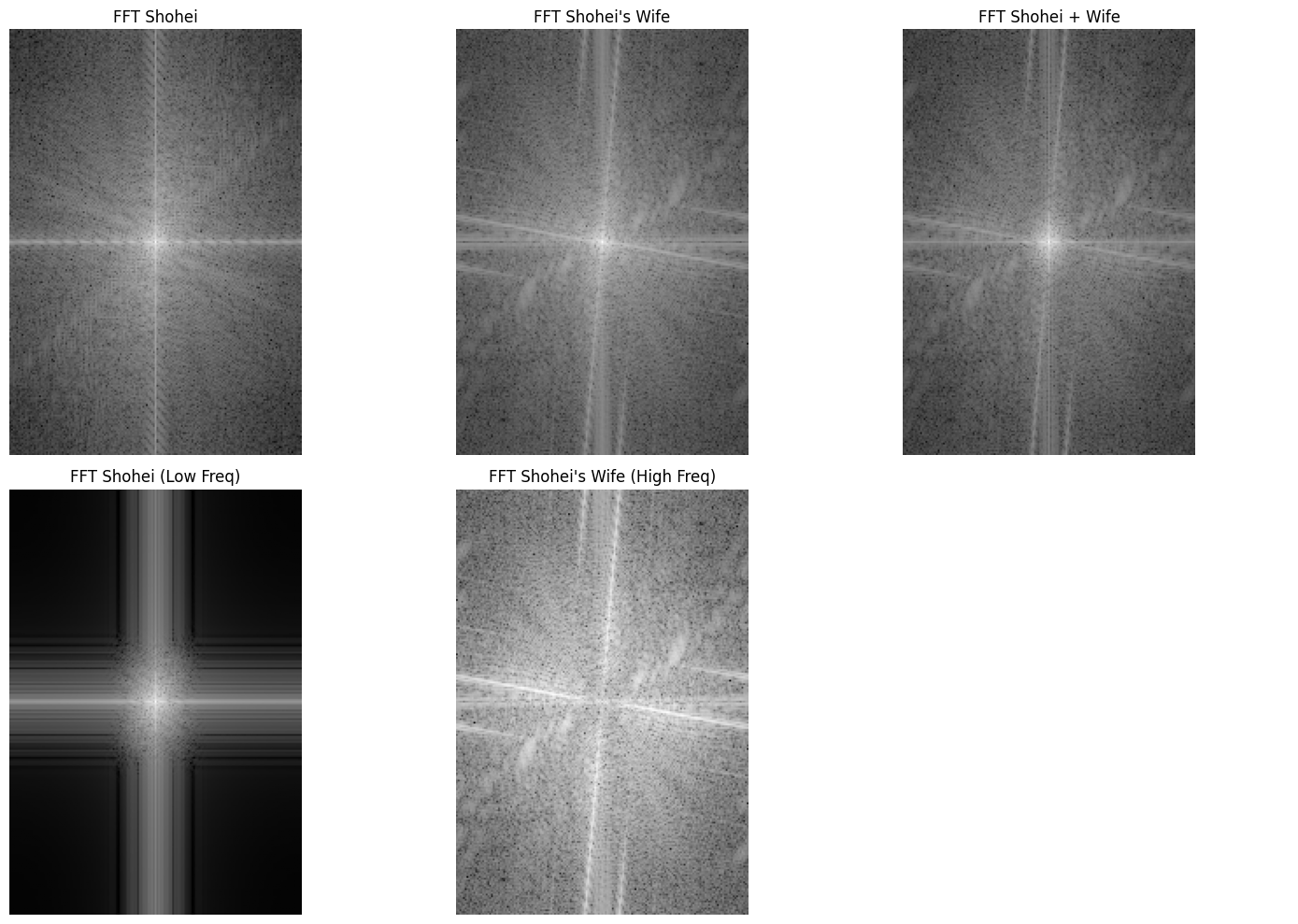
2.2.6 Shohei Ohtani + Wife
Parameters: σlow=3, σhigh=1.3
Observations
- The frequency response plots show the separation of low and high frequencies, though the high-frequency center doesn't appear as dark as expected (maybe due to visualization scaling?)
Part 2.3: Gaussian and Laplacian Stacks
Unlike Gaussian pyramids which downsample at each level (as seen in Project 1), Gaussian stacks keep all levels at the same resolution as the original image. This makes them ideal for multi-resolution blending.
Stack vs Pyramid
Gaussian Pyramid (Project 1):
- Each level is downsampled (half size)
- Used for efficient processing
- Different resolutions at each level
Gaussian Stack (This Project):
- All levels keep same size as original
- No downsampling, just increasing blur
- Essential for multi-resolution blending
2.3.1 Building Gaussian Stack
At each level, we apply progressively stronger Gaussian blur while maintaining the original image size:
Gaussian Stack Implementation
[Common Pitfall] Blur the previous level repeatedly
- Level 1: Blur original with σ=2
- Level 2: Blur Level 1 with σ=4 → cumulative blur exceeds σ=4
- Level 3: Blur Level 2 with σ=8 → cumulative blur far exceeds σ=8
- Result: Compounding blur that grows much faster than exponential
2.3.2 Building Laplacian Stack
The Laplacian stack captures the difference between consecutive Gaussian levels, representing different frequency bands. Note that the last layer is directly taken from the Gaussian stack's last layer (not a difference), as there's no next level to subtract.
Laplacian Stack Implementation
Why does the last Laplacian layer = last Gaussian layer?
In a Laplacian stack, each layer represents a frequency band extracted as the difference between consecutive Gaussian levels. However, the last layer has no next level to subtract from, so we keep the final Gaussian layer as-is. This represents the lowest frequency band (most blurred version) of the image.
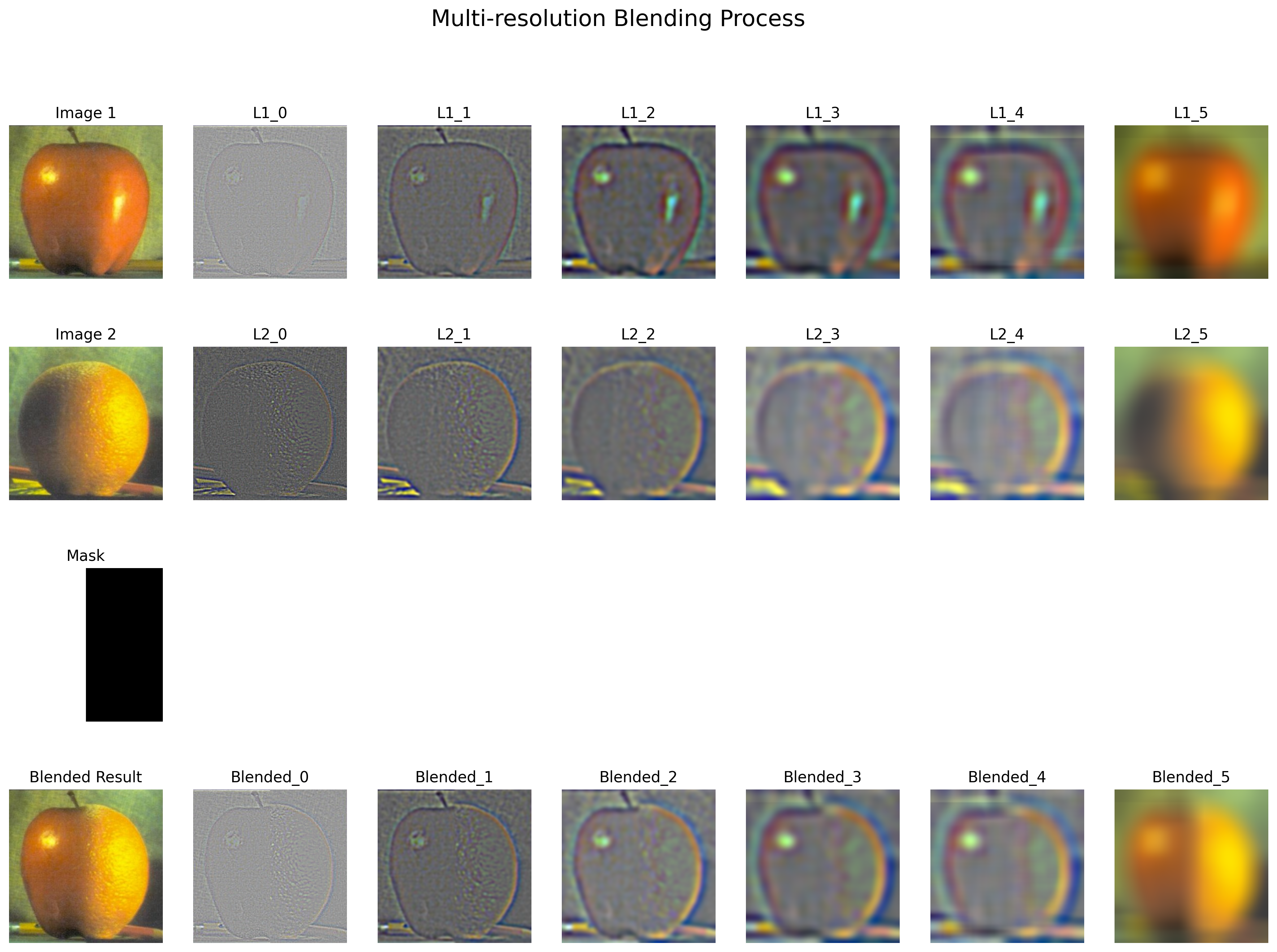
2.3.3 Results: Apple and Orange Stacks
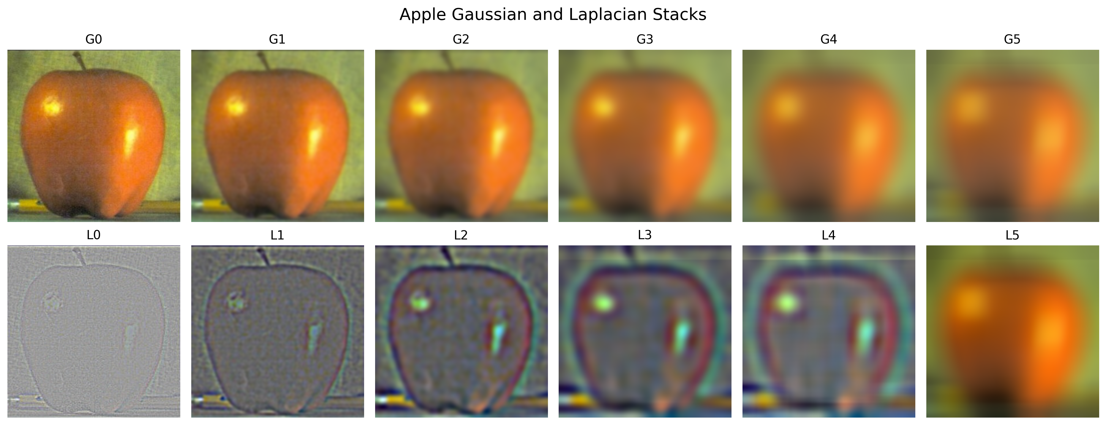
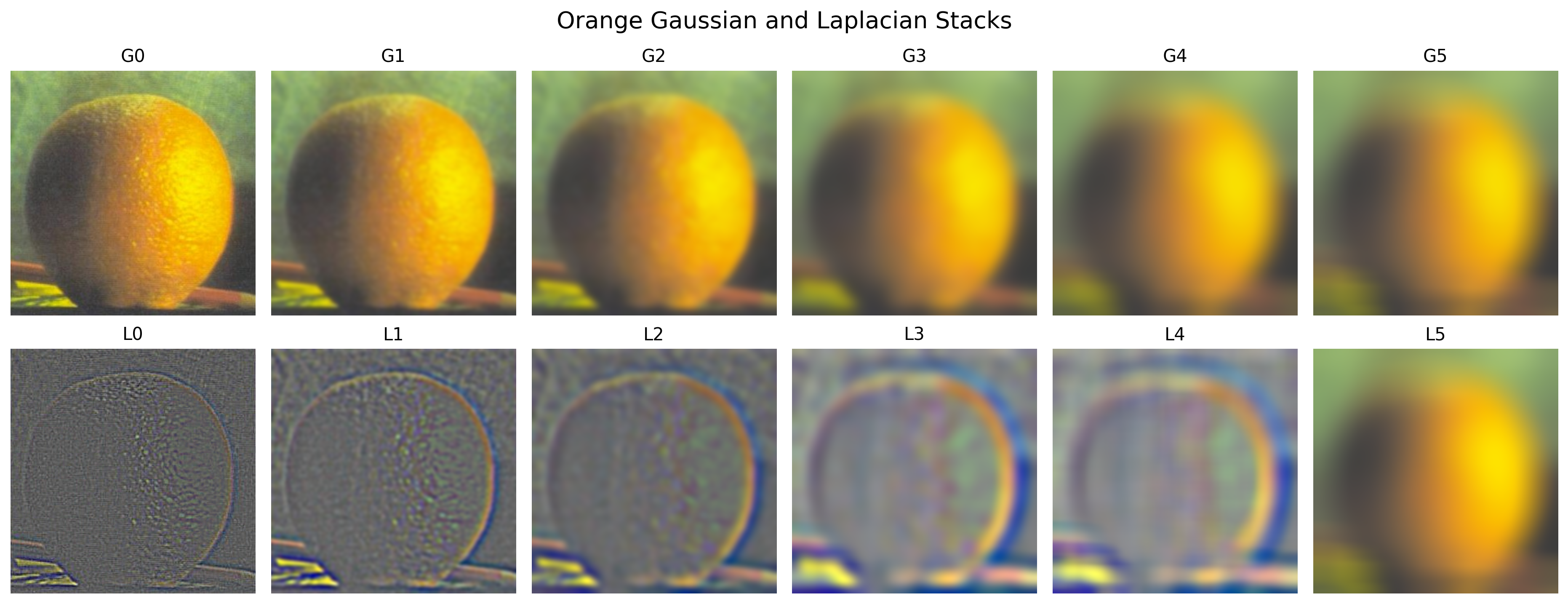
I built 6-level Gaussian and Laplacian stacks for both apple and orange images:
Observations
- Gaussian Stack: Each level becomes more blurred while maintaining full resolution
- Laplacian Stack: Each layer (except the last) captures a specific frequency band, appearing mostly gray with edges highlighted
- Last Laplacian layer: Contains the low-frequency content (blurry version), identical to the last Gaussian layer
Part 2.4: Multi-resolution Blending
Multi-resolution blending uses Laplacian stacks to seamlessly combine images at different frequency bands, avoiding harsh transitions. By blending each frequency level separately with a smoothly transitioning mask, we achieve natural-looking composites.
2.4.1 Image Selection
I selected three pairs of images to blend using different mask shapes:
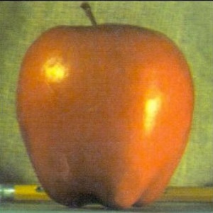
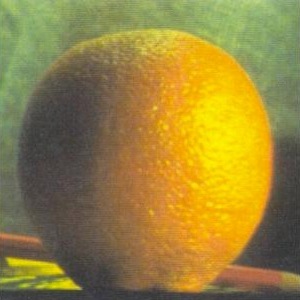
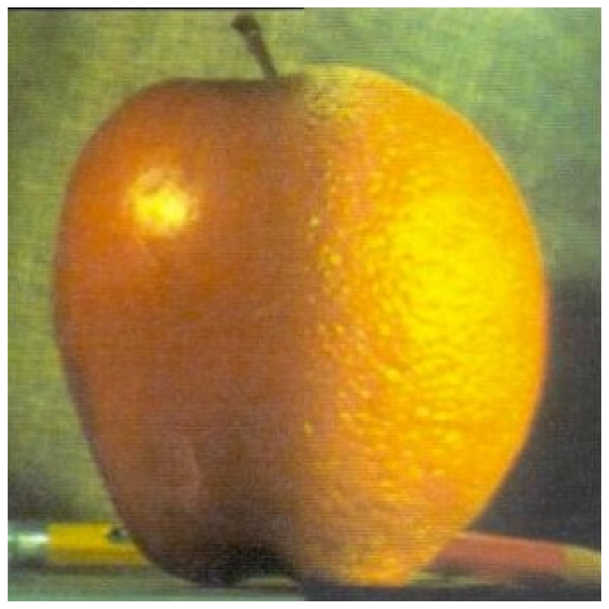
Apple + Orange
The classic oraple from project spec.
Jay Chou + Me
It will be a good idea to blend this picture again since it has similar background and position!
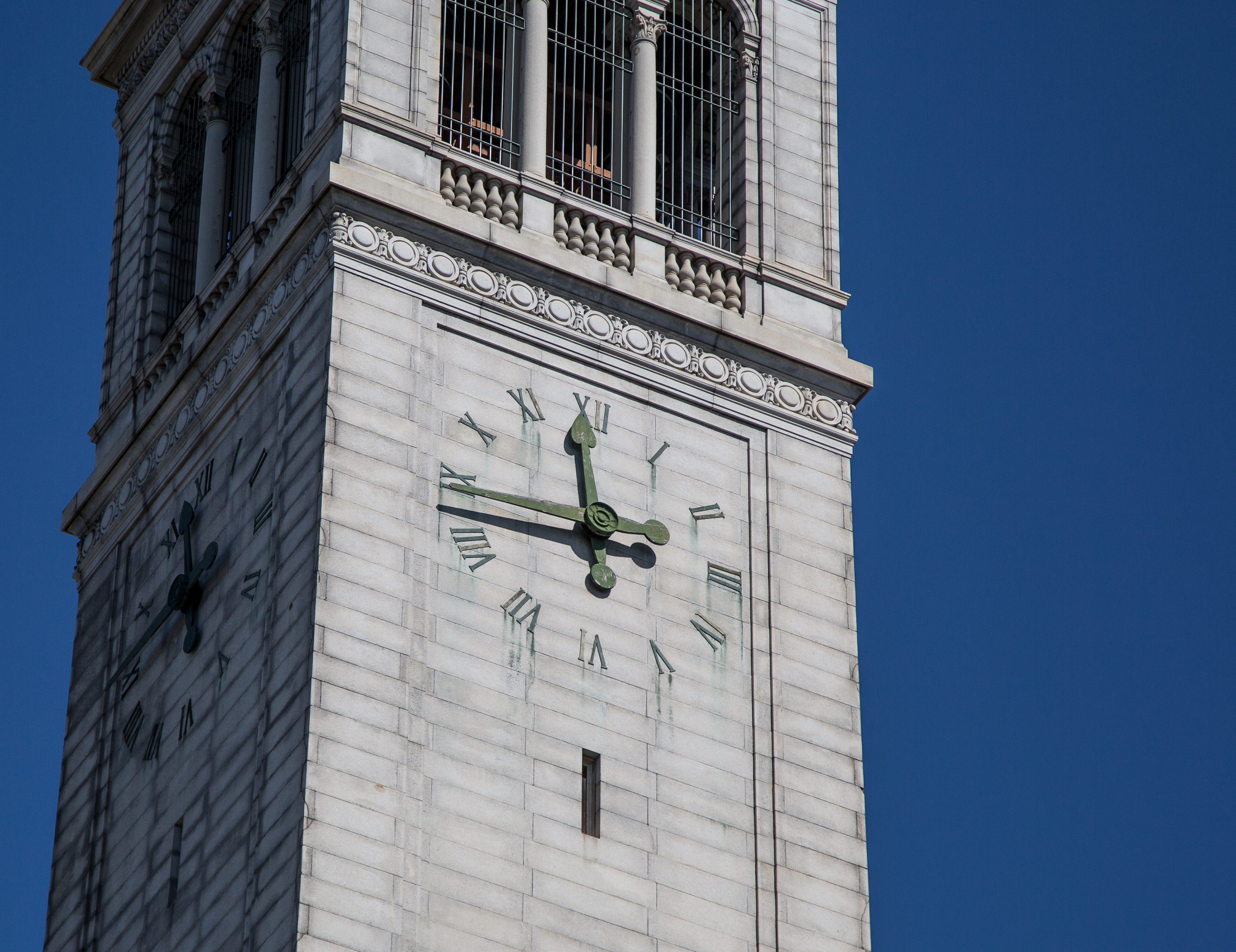
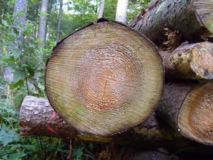
Campanile + Tree Rings
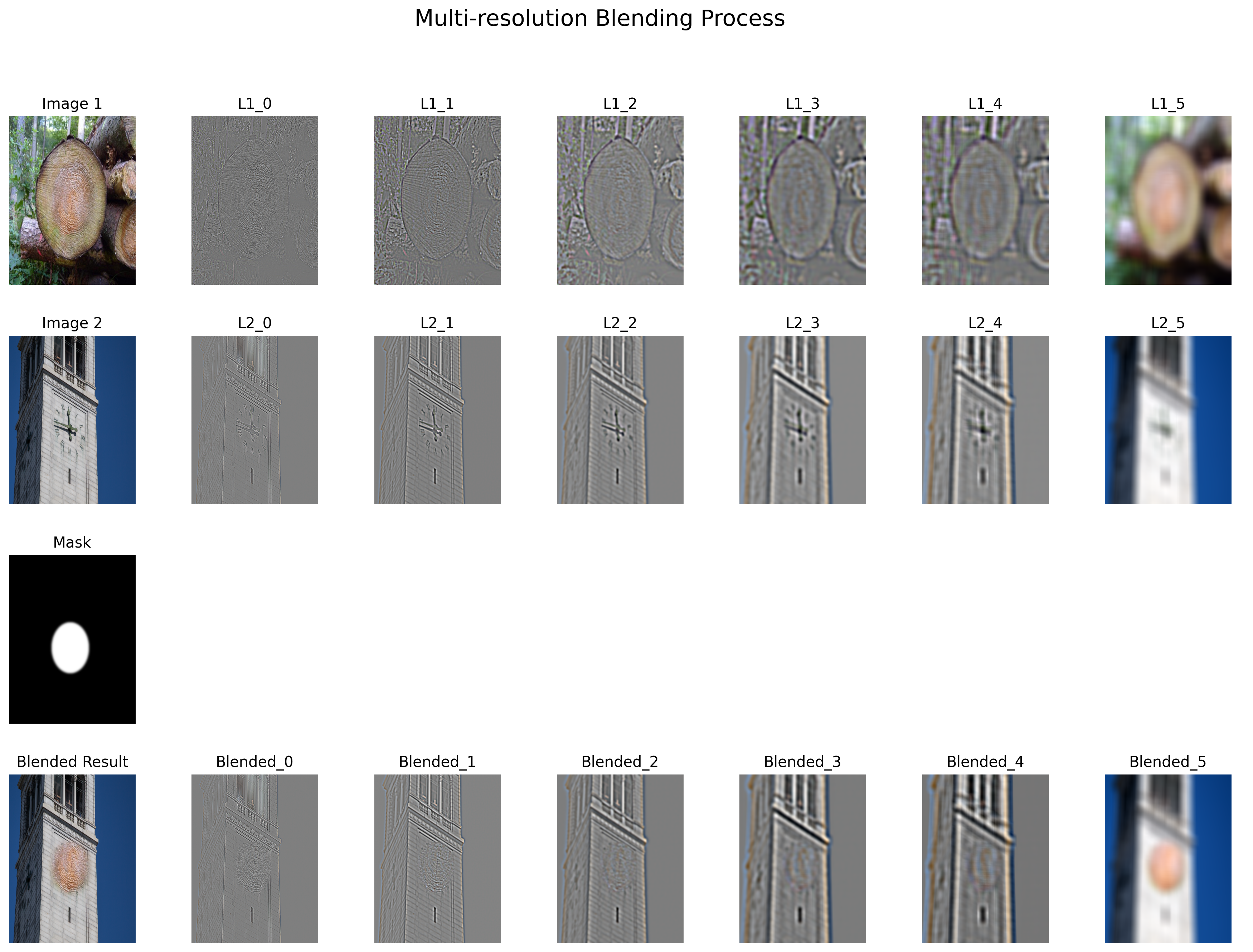
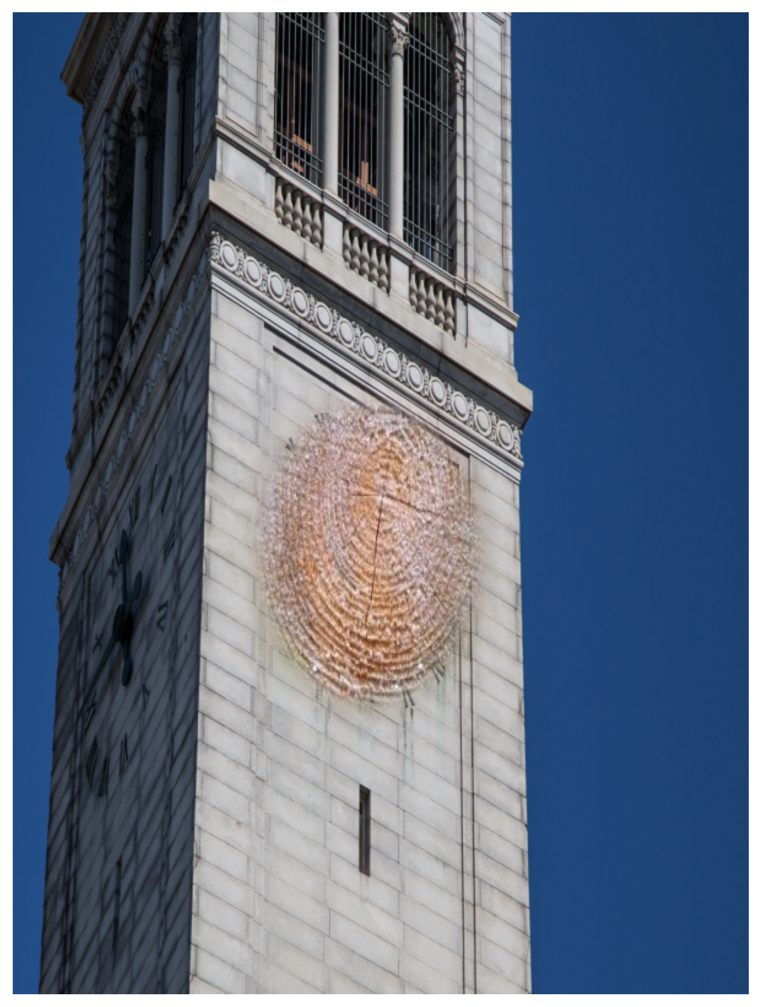
I spent many days thinking about what to blend. Then while walking past the campanile, I realized: why not blend tree rings into the tower? It needs an irregular mask anyway!
(Photos sourced online)
2.4.2 Implementation: Masks and Blending
I implemented four types of masks for different blending scenarios:
Mask Creation Functions
Multi-resolution Blending Function
2.4.3 Apple + Orange (Vertical Mask)
Parameters: create_vertical_mask(split_ratio=0.5), levels=6
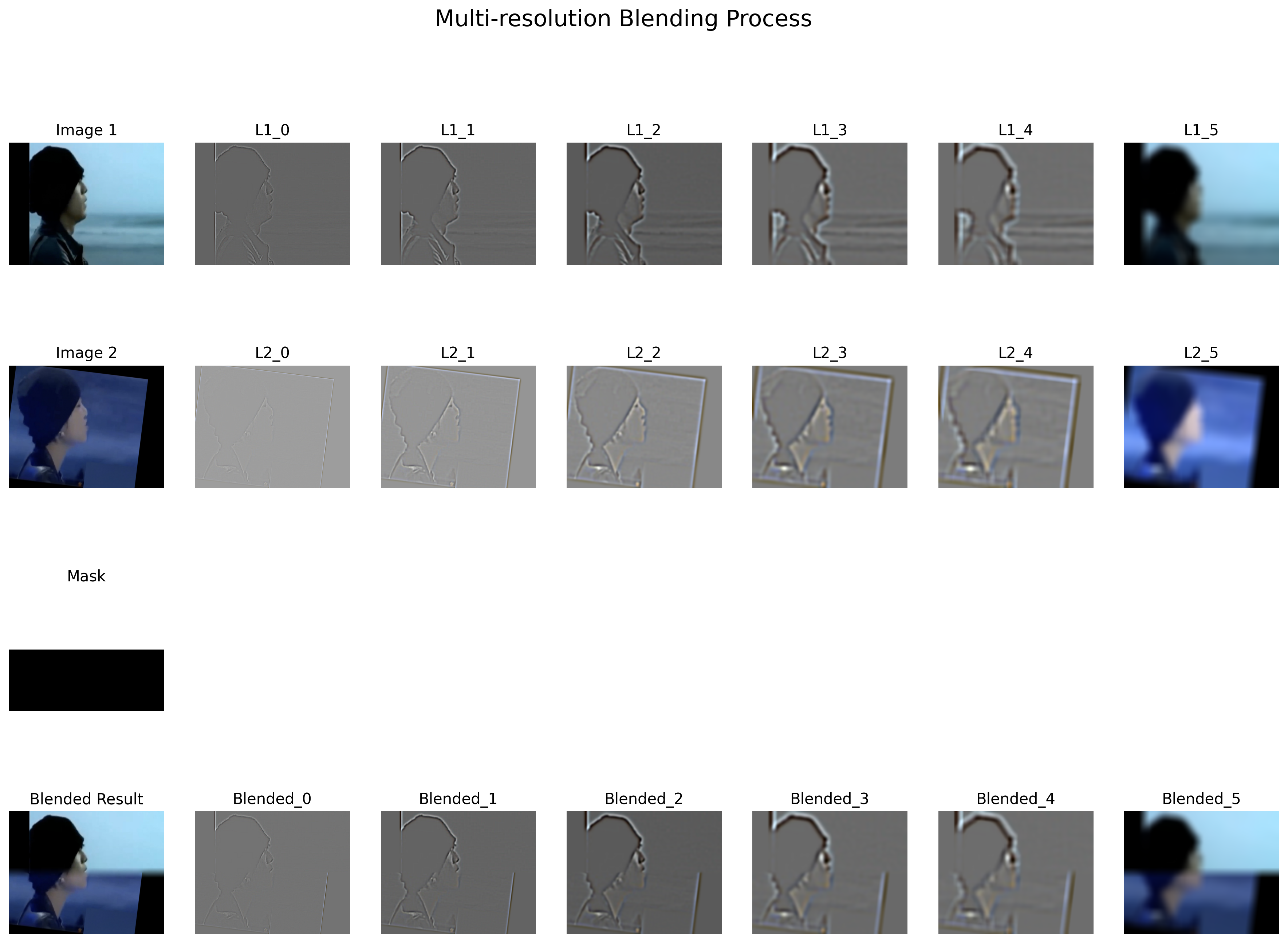
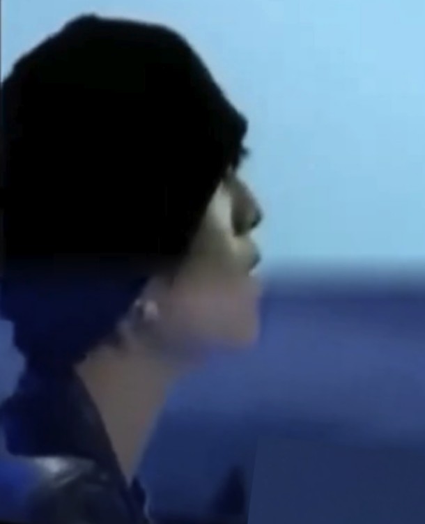
2.4.4 Jay Chou + Me (Horizontal Mask)
Parameters: create_horizontal_mask(split_ratio=0.5), levels=6
2.4.5 Campanile + Tree Rings (Ellipse Mask)
Parameters: Both images resized to 800×600, create_ellipse_mask(center=(440, 290), radius_x=89, radius_y=121), levels=6