Part A.2: Recover Homographies
Compute the homography matrix H that maps points from one image to another.
💻 Best viewed on desktop (1920×1080 or larger) for optimal experience
Manually select correspondences, compute homographies, warp images, and blend them into seamless panoramas.
Automatically detect Harris corners, extract MOPS descriptors, match features using Lowe's ratio test, and robustly compute homographies with RANSAC.
I captured two sets of images with projective transformations by fixing the center of projection (COP) and rotating the camera while keeping the same position.
iPhone 14 Pro 1× lens
(avoid barrel distortion by not using fisheye)
40~70%
Too little overlap makes registration harder.
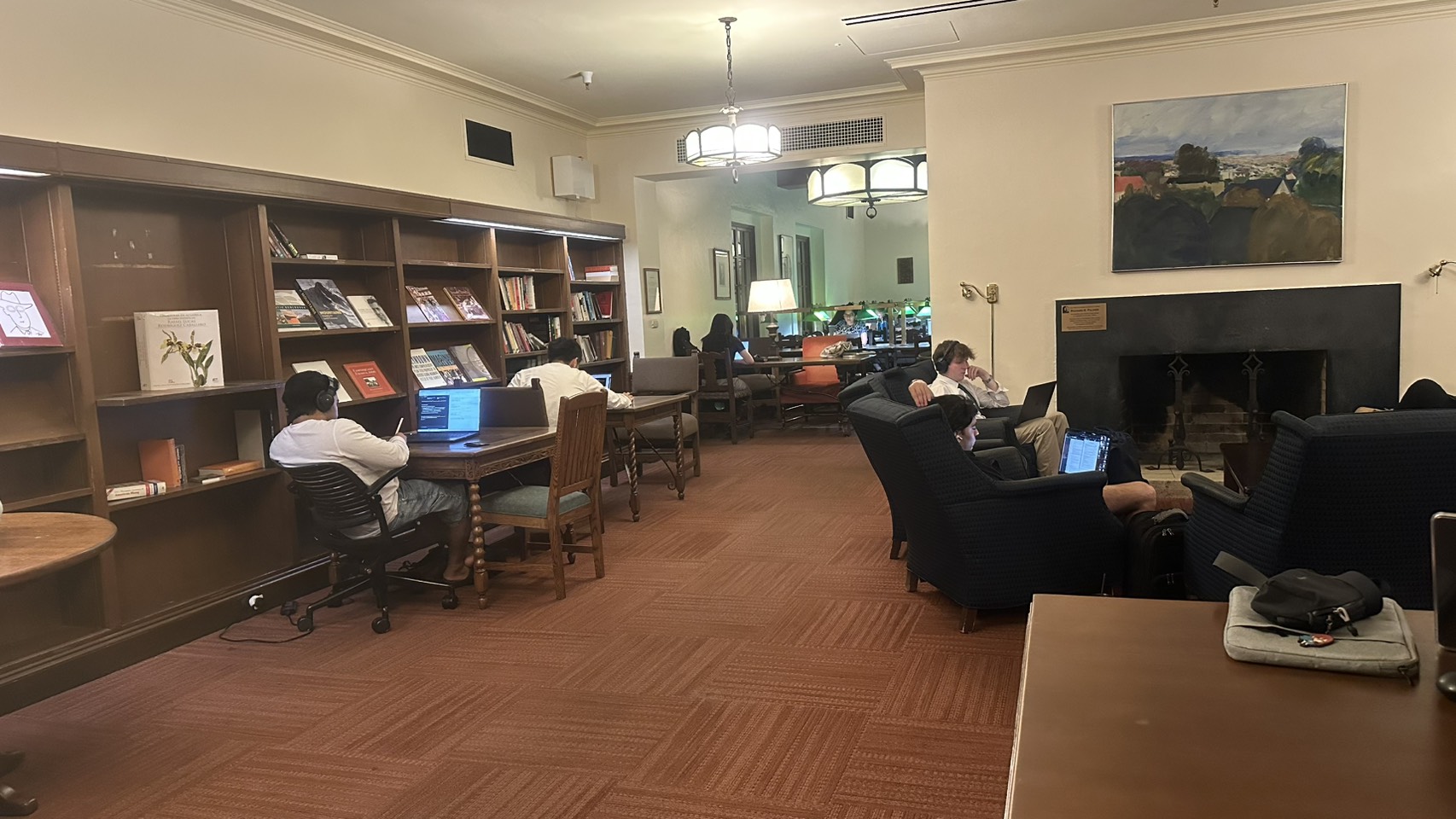
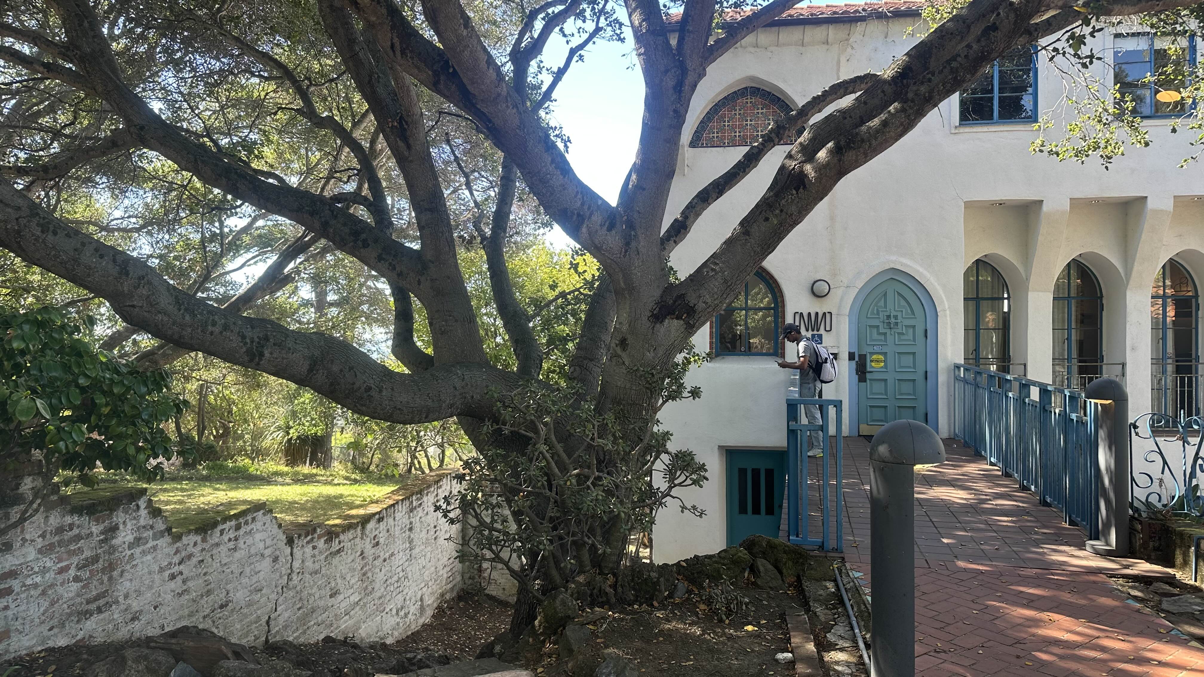
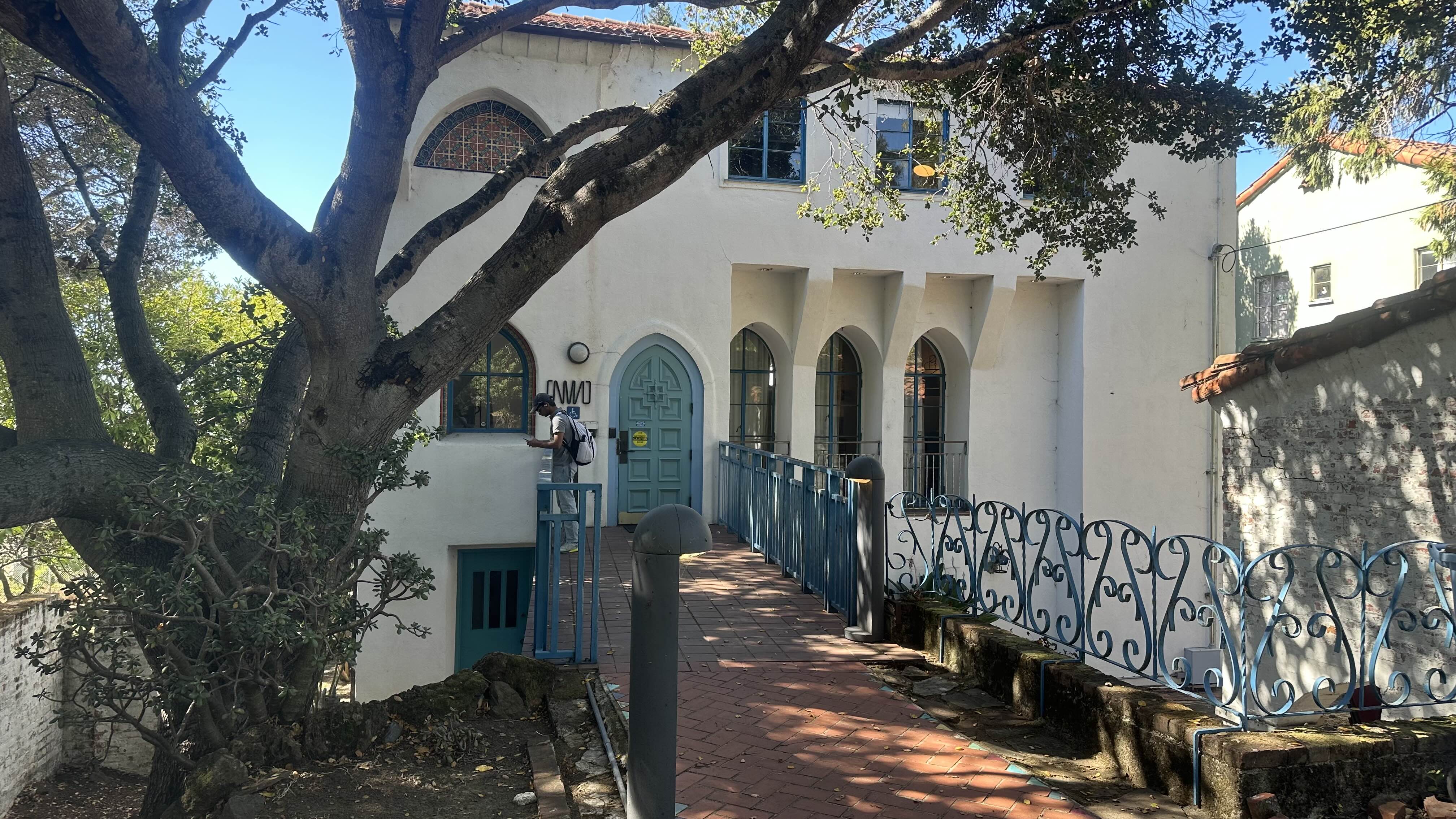
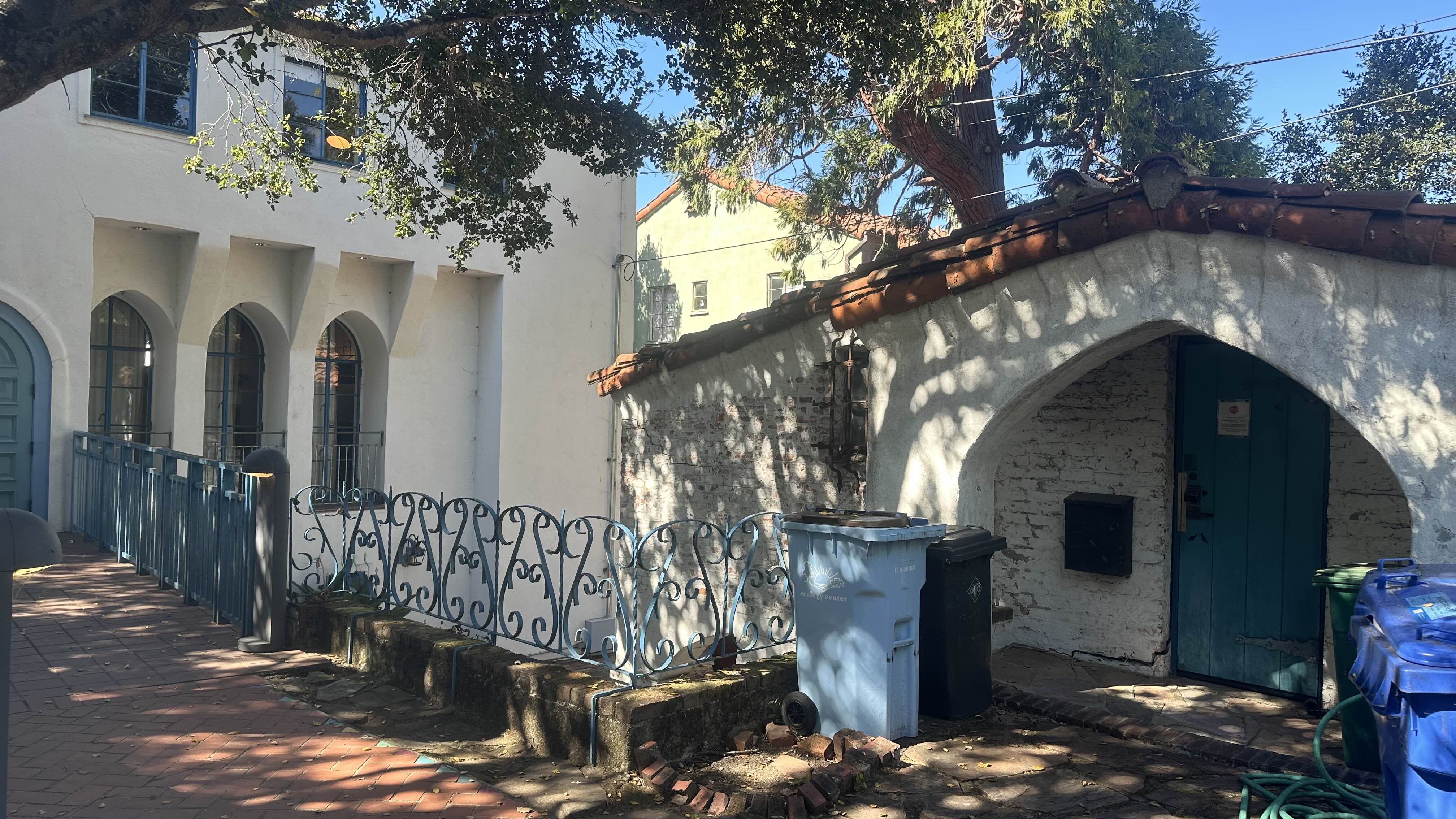
This is where I spent most of my time during my exchange year in UC Berkeley.
🖱️ Scroll to navigate through images horizontally
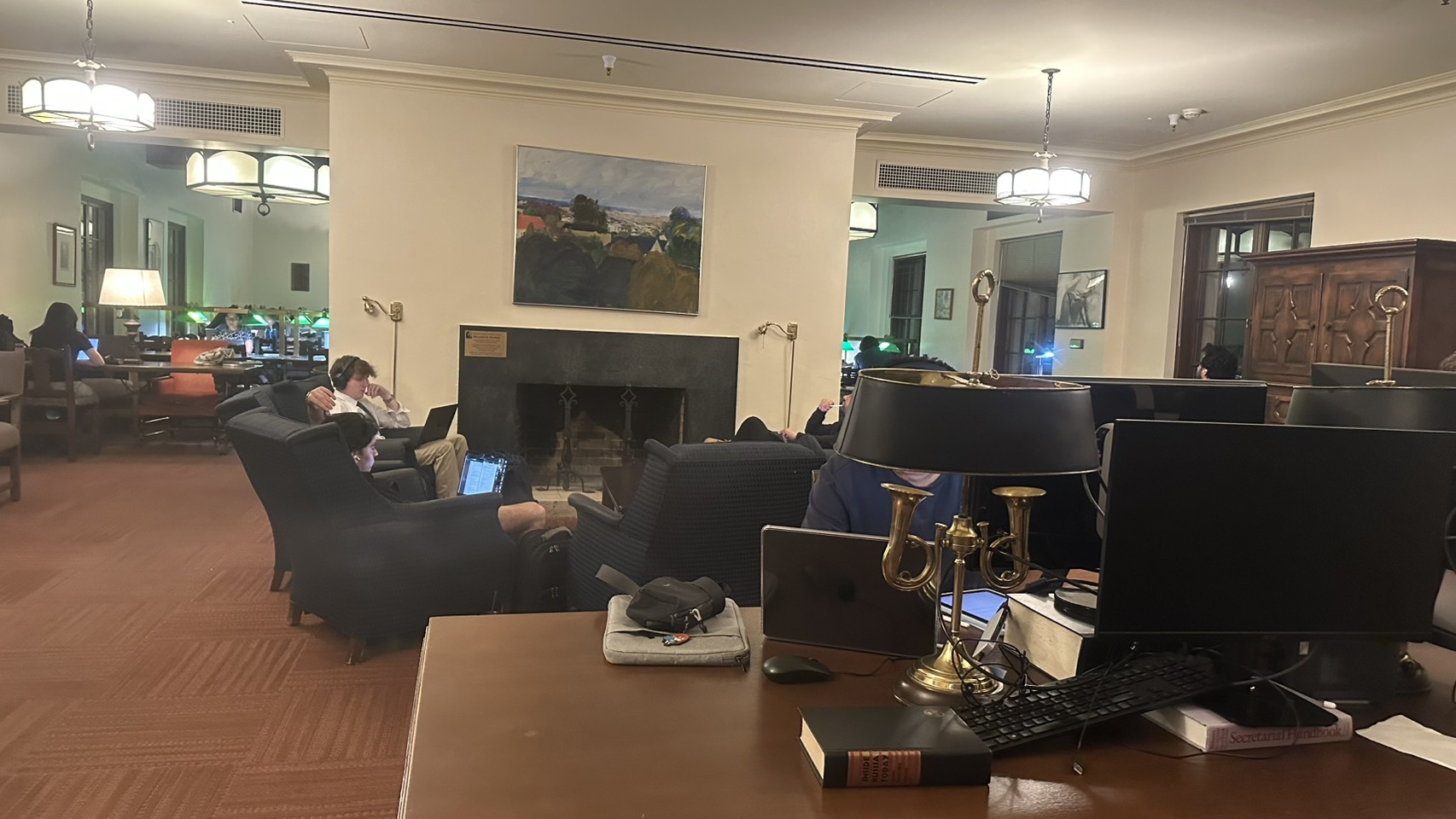
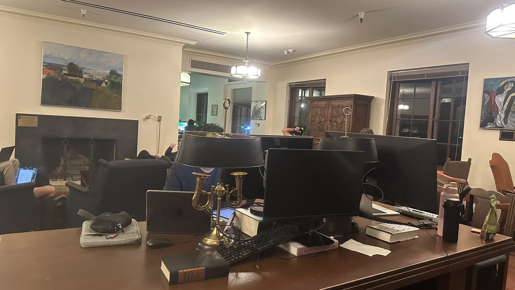
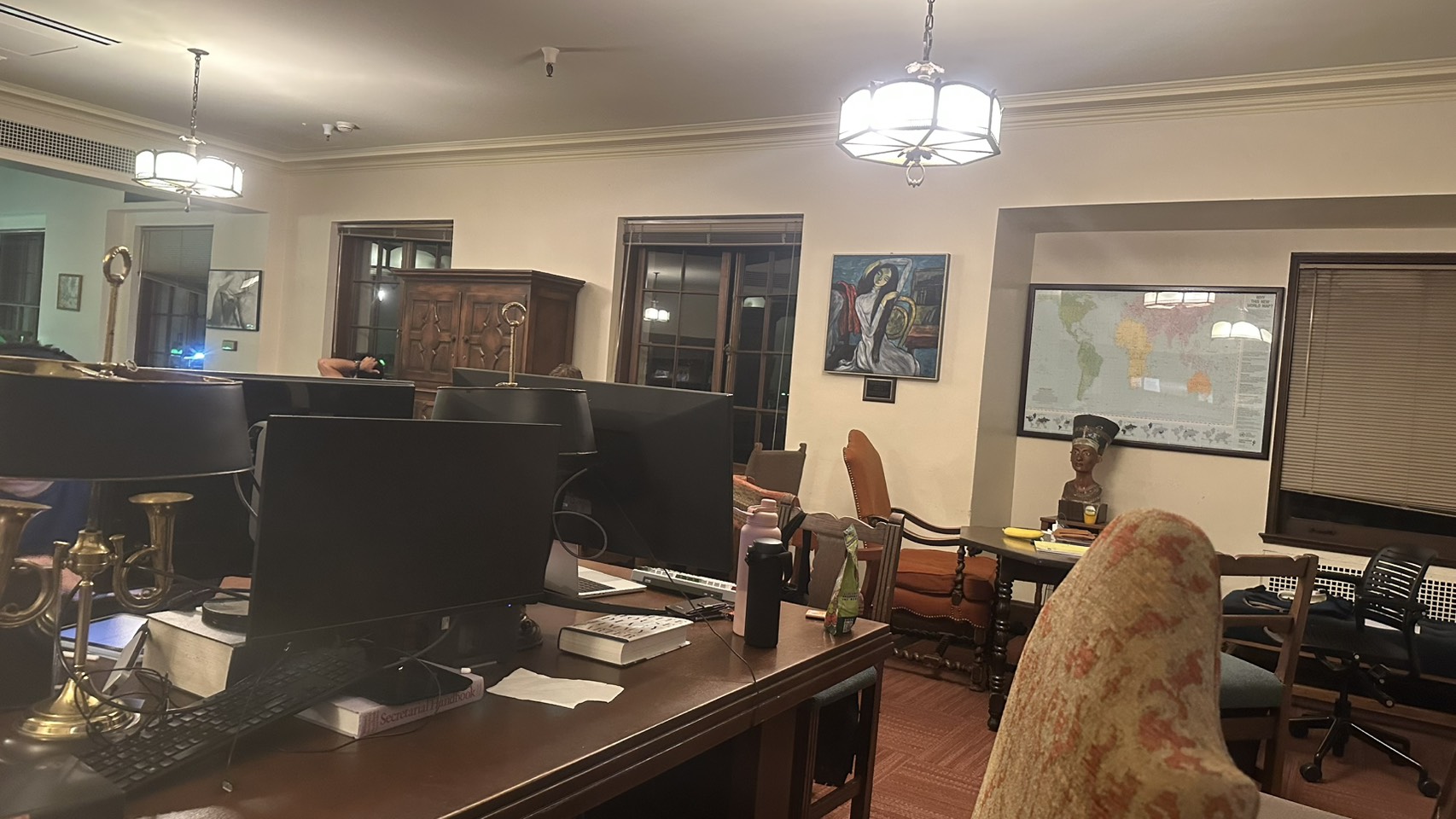
This location is meaningful to me as it's where I conducted my undergraduate research.
🖱️ Scroll to navigate through images horizontally
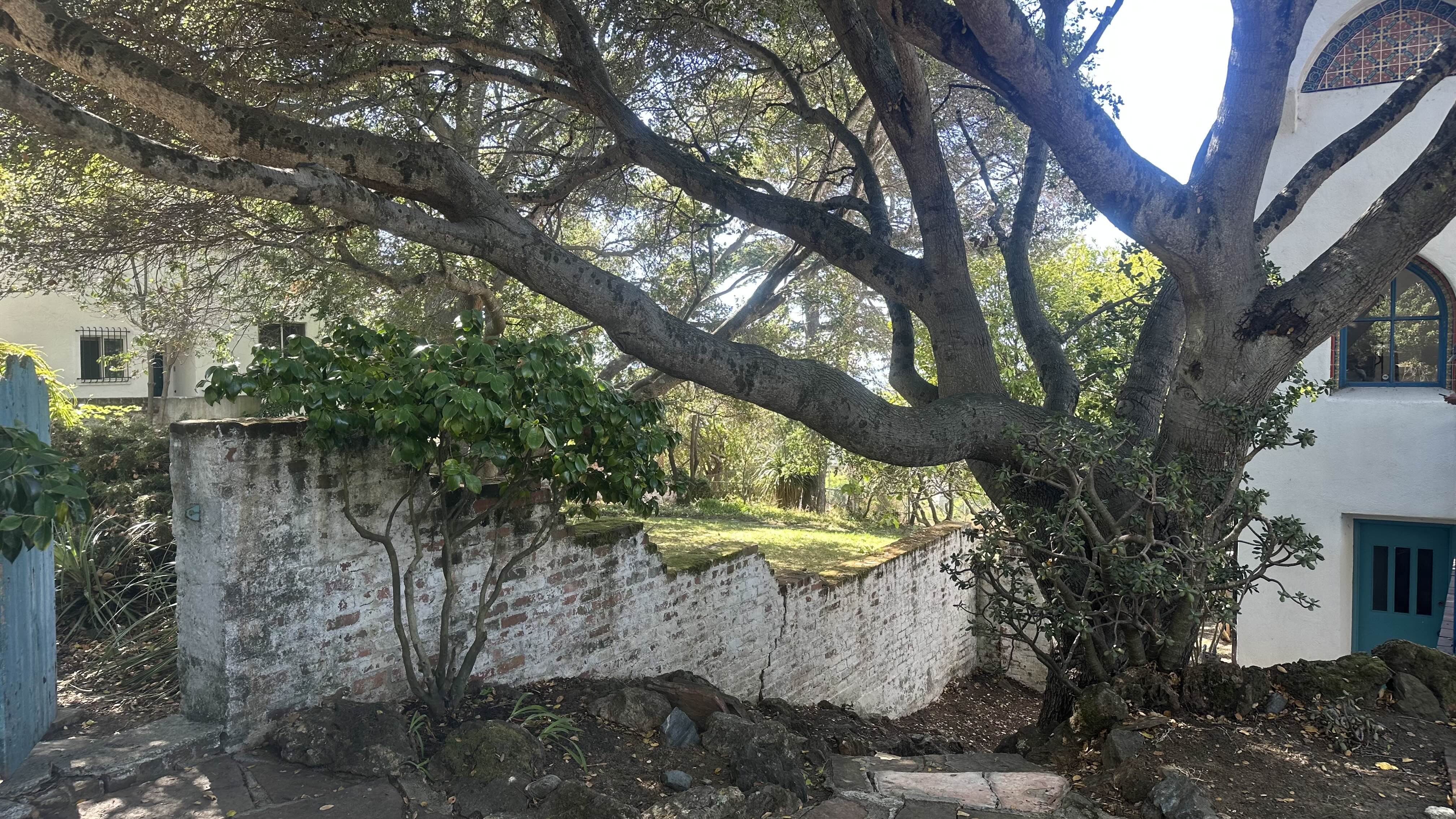
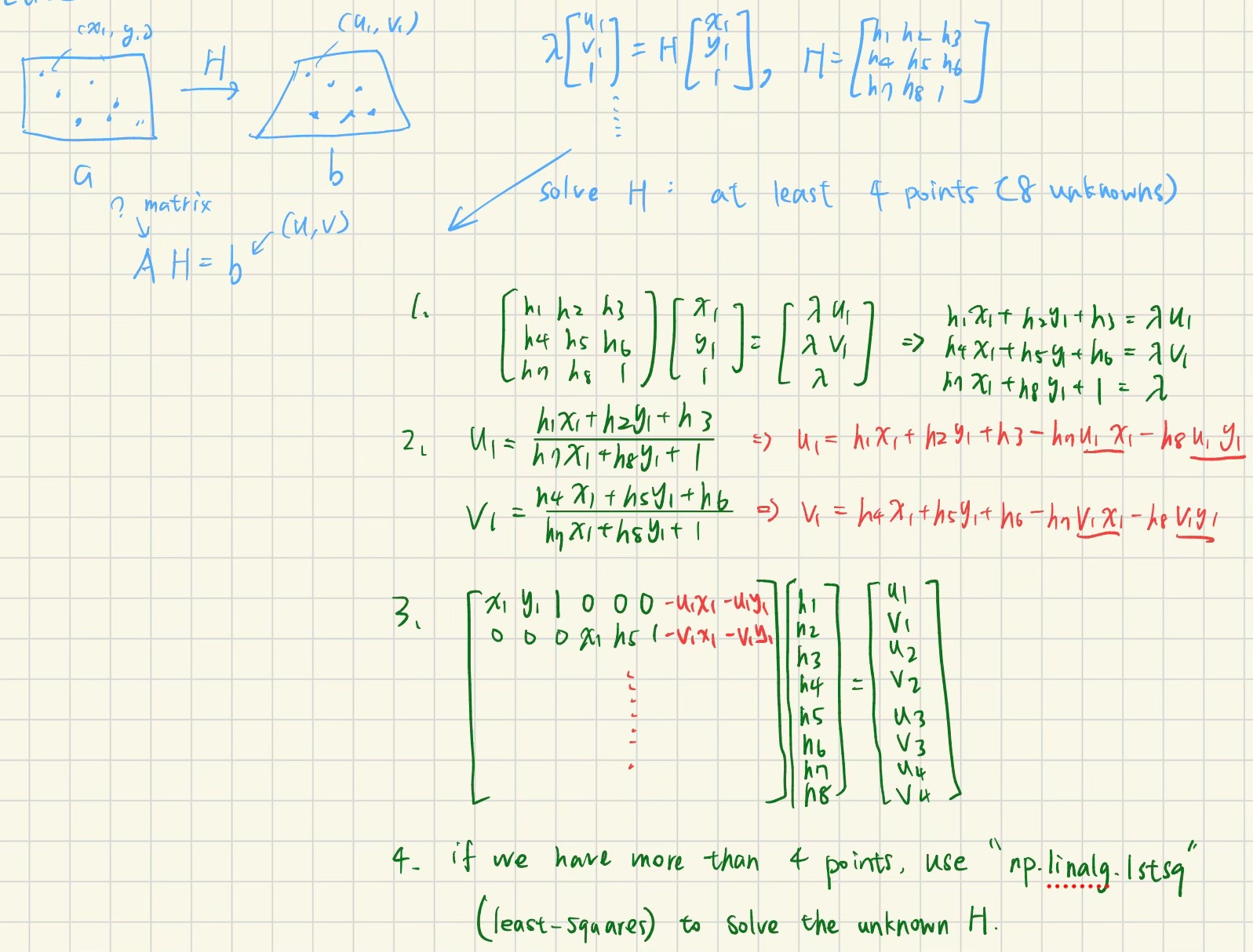
Compute the homography matrix H that maps points from one image to another.
For each correspondence pair (x, y) ↔ (u, v), we construct two linear equations:
h₁x + h₂y + h₃ - h₇ux - h₈uy = uh₄x + h₅y + h₆ - h₇vx - h₈vy = vWith n correspondence points, we build the system Ah = b where:
A is a 2n × 8 matrix containing the coordinates and their productsh is an 8 × 1 vector of unknown homography coefficientsb is a 2n × 1 vector of target coordinatesWe solve this using least-squares: h = (AᵀA)⁻¹Aᵀb, then reconstruct the 3×3 homography matrix with h₉ = 1.
computeH
# File: part2_homography.py:69-92

def computeH(pts1, pts2):
    n = len(pts1)
    A = np.zeros((2*n, 8))
    b = np.zeros((2*n, 1))

    for i in range(n):
        x, y = pts1[i]
        u, v = pts2[i]

        A[2*i] = [x, y, 1, 0, 0, 0, -u*x, -u*y]
        b[2*i] = u

        A[2*i+1] = [0, 0, 0, x, y, 1, -v*x, -v*y]
        b[2*i+1] = v

    h, _, _, _ = np.linalg.lstsq(A, b, rcond=None)

    H = np.zeros((3, 3))
    H[0, :] = h[:3].flatten()
    H[1, :] = h[3:6].flatten()
    H[2, :2] = h[6:].flatten()
    H[2, 2] = 1

return H, A, bpart2_homography.py)
select_correspondences() — Interactive point selection using matplotlib ginputvisualize_correspondences() — Draws correspondences on image pairssave_correspondences(), load_correspondences() — Save and load selected points in json to avoid re-selectingverify_homography(), print_system() — Displays the linear system and compute reprojection error for website demopart2_exec.py)
An interactive CLI to detect the scene from images folder, choose which two images to process, decide how many correspondence points to mark, automatically save correspondences for future use
Using the interactive script, by selecting "ihouse-library" folder and picture 1 and 2, we manually click the points:
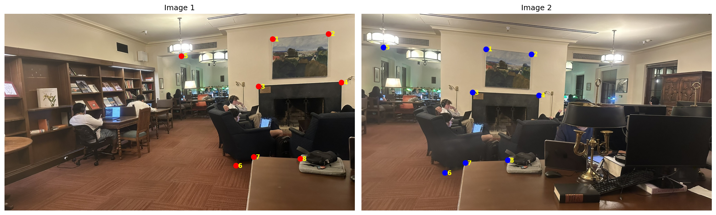
Then, we get the (x,y) and (u,v), which can be written as the form matrix A (16×8) and b (16×1). Let's do computeH():
First 4 rows of A:
[[ 1.305e+03  1.229e+02  1.000e+00  0.000e+00 0.000e+00  0.000e+00 -7.926e+05 -7.462e+04]
 [ 0.000e+00  0.000e+00  0.000e+00  1.305e+03 1.229e+02  1.000e+00 -2.245e+05 -2.113e+04]
 [ 1.578e+03  9.773e+01  1.000e+00  0.000e+00 0.000e+00  0.000e+00 -1.306e+06 -8.086e+04]
 [ 0.000e+00  0.000e+00  0.000e+00  1.578e+03 9.773e+01  1.000e+00 -3.111e+05 -1.926e+04]
                                        ...                                             ]

First 4 rows of b:
[607.18
 171.96
 827.34
 197.12
  ...  ]
[[ 2.916e+00]
 [-1.578e-01]
 [-2.272e+03]
 [ 6.617e-01]
 [ 2.247e+00]
 [-7.104e+02]
 [ 1.153e-03]
 [-1.504e-04]]


Mean error: 2.45 pixels
Max error: 3.22 pixelsIn this part, we apply our Homography transformation in Part A.2 and warp two additional rectangle items using inverse warping with nearest neighbor and bilinear interpolation for vertification.
For each pixel (u, v) in our desired output image, we compute the corresponding source location using:
[x_i, y_i, 1]ᵀ = H⁻¹ · [u, v, 1]ᵀ(x, y) = (x_i/w, y_i/w) where w is the homogeneous coordinateRound to the nearest integer coordinates:
x' = round(x), y' = round(y)output[u,v] = input[y', x']Weighted average of 4 neighboring pixels:
x₀ = ⌊x⌋, y₀ = ⌊y⌋dx = x - x₀, dy = y - y₀w₀₀ = (1-dx)(1-dy)w₀₁ = (1-dx)·dyw₁₀ = dx·(1-dy)w₁₁ = dx·dy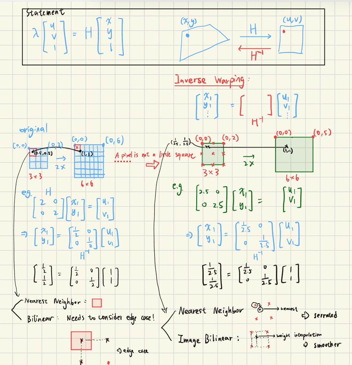
warpImageNearestNeighbor
def warpImageNearestNeighbor(im, H, output_shape=None):
    h, w = im.shape[:2]
    has_color = len(im.shape) == 3

    if output_shape is None:
        out_h, out_w, offset = compute_output_bounds(im.shape, H)
        T_offset = np.array([
            [1, 0, -offset[0]],
            [0, 1, -offset[1]],
            [0, 0, 1]
        ])
        H_adjusted = T_offset @ H
    else:
        out_h, out_w = output_shape
        H_adjusted = H

    if has_color:
        out_im = np.zeros((out_h, out_w, im.shape[2]))
    else:
        out_im = np.zeros((out_h, out_w))
    alpha = np.zeros((out_h, out_w))

    H_inv = np.linalg.inv(H_adjusted)

    y_coords, x_coords = np.meshgrid(np.arange(out_h), np.arange(out_w), indexing='ij')
    coords = np.stack([x_coords, y_coords, np.ones_like(x_coords)], axis=-1)

    src_h = coords @ H_inv.T
    denom = src_h[..., 2]

    with np.errstate(divide='ignore', invalid='ignore'):
        src_coords = src_h[..., :2] / denom[..., np.newaxis]

    safe_denom = np.isfinite(src_coords).all(axis=-1)

    src_x = np.round(src_coords[..., 0]).astype(int)
    src_y = np.round(src_coords[..., 1]).astype(int)

    valid = safe_denom & (src_x >= 0) & (src_x < w) & (src_y >= 0) & (src_y < h)
    out_im[valid] = im[src_y[valid], src_x[valid]]
    alpha[valid] = 1

    if has_color:
        result = np.zeros((out_h, out_w, 4), dtype=out_im.dtype)
        result[..., :3] = out_im
        result[..., 3] = alpha
    else:
        result = np.zeros((out_h, out_w, 2), dtype=out_im.dtype)
        result[..., 0] = out_im
        result[..., 1] = alpha

return resultwarpImageBilinear
def warpImageBilinear(im, H, output_shape=None):
    h, w = im.shape[:2]
    has_color = len(im.shape) == 3

    if output_shape is None:
        out_h, out_w, offset = compute_output_bounds(im.shape, H)
        T_offset = np.array([
            [1, 0, -offset[0]],
            [0, 1, -offset[1]],
            [0, 0, 1]
        ])
        H_adjusted = T_offset @ H
    else:
        out_h, out_w = output_shape
        H_adjusted = H

    if has_color:
        out_im = np.zeros((out_h, out_w, im.shape[2]))
    else:
        out_im = np.zeros((out_h, out_w))
    alpha = np.zeros((out_h, out_w))

    H_inv = np.linalg.inv(H_adjusted)

    y_coords, x_coords = np.meshgrid(np.arange(out_h), np.arange(out_w), indexing='ij')
    coords = np.stack([x_coords, y_coords, np.ones_like(x_coords)], axis=-1)

    src_h = coords @ H_inv.T
    denom = src_h[..., 2]

    with np.errstate(divide='ignore', invalid='ignore'):
        src_coords = src_h[..., :2] / denom[..., np.newaxis]

    safe_denom = np.isfinite(src_coords).all(axis=-1)

    src_x = src_coords[..., 0]
    src_y = src_coords[..., 1]

    x0 = np.floor(src_x).astype(int)
    x1 = x0 + 1
    y0 = np.floor(src_y).astype(int)
    y1 = y0 + 1

    valid = safe_denom & (x0 >= 0) & (x1 < w) & (y0 >= 0) & (y1 < h)

    dx = src_x - x0
    dy = src_y - y0

    w00 = (1 - dx) * (1 - dy)
    w01 = (1 - dx) * dy
    w10 = dx * (1 - dy)
    w11 = dx * dy

    if has_color:
        out_im[valid] = (
            w00[valid, np.newaxis] * im[y0[valid], x0[valid]] +
            w01[valid, np.newaxis] * im[y1[valid], x0[valid]] +
            w10[valid, np.newaxis] * im[y0[valid], x1[valid]] +
            w11[valid, np.newaxis] * im[y1[valid], x1[valid]]
        )
    else:
        out_im[valid] = (
            w00[valid] * im[y0[valid], x0[valid]] +
            w01[valid] * im[y1[valid], x0[valid]] +
            w10[valid] * im[y0[valid], x1[valid]] +
            w11[valid] * im[y1[valid], x1[valid]]
        )

    alpha[valid] = 1

    if has_color:
        result = np.zeros((out_h, out_w, 4), dtype=out_im.dtype)
        result[..., :3] = out_im
        result[..., 3] = alpha
    else:
        result = np.zeros((out_h, out_w, 2), dtype=out_im.dtype)
        result[..., 0] = out_im
        result[..., 1] = alpha

return resultcompute_output_bounds
def compute_output_bounds(im_shape, H):
    h, w = im_shape[:2]
    corners = np.array([
        [0, 0, 1],
        [w-1, 0, 1],
        [0, h-1, 1],
        [w-1, h-1, 1]
    ])

    warped_corners = (H @ corners.T).T
    warped_corners = warped_corners[:, :2] / warped_corners[:, 2:3]

    min_x_i = int(np.floor(warped_corners[:, 0].min()))
    min_y_i = int(np.floor(warped_corners[:, 1].min()))
    max_x_i = int(np.ceil(warped_corners[:, 0].max()))
    max_y_i = int(np.ceil(warped_corners[:, 1].max()))

    out_w = (max_x_i - min_x_i) + 1
    out_h = (max_y_i - min_y_i) + 1

    offset = np.array([min_x_i, min_y_i])

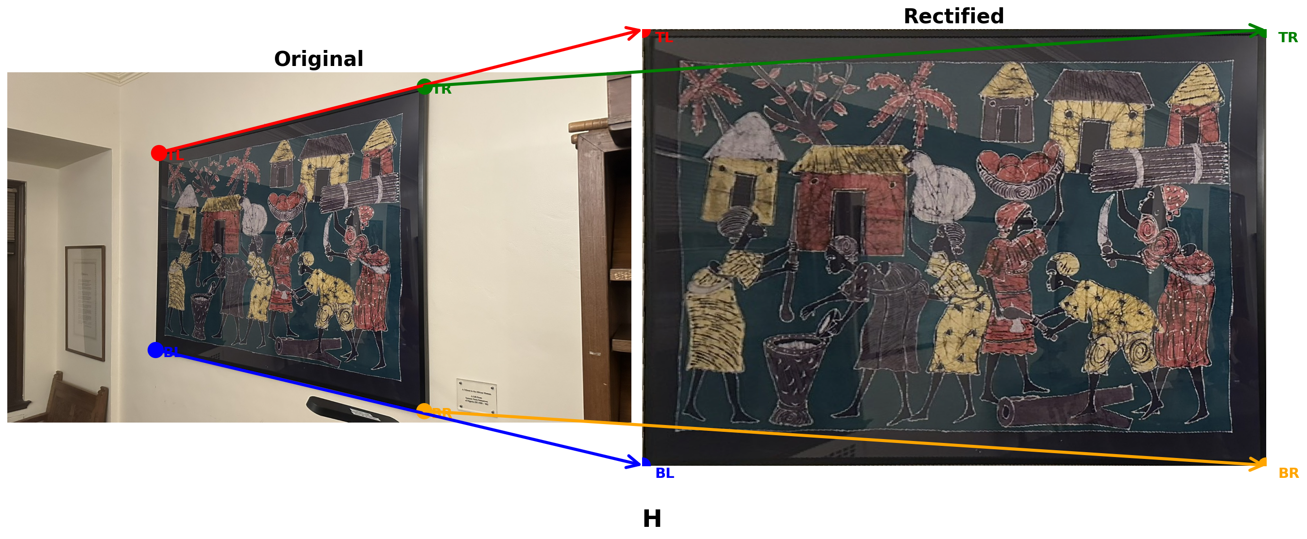
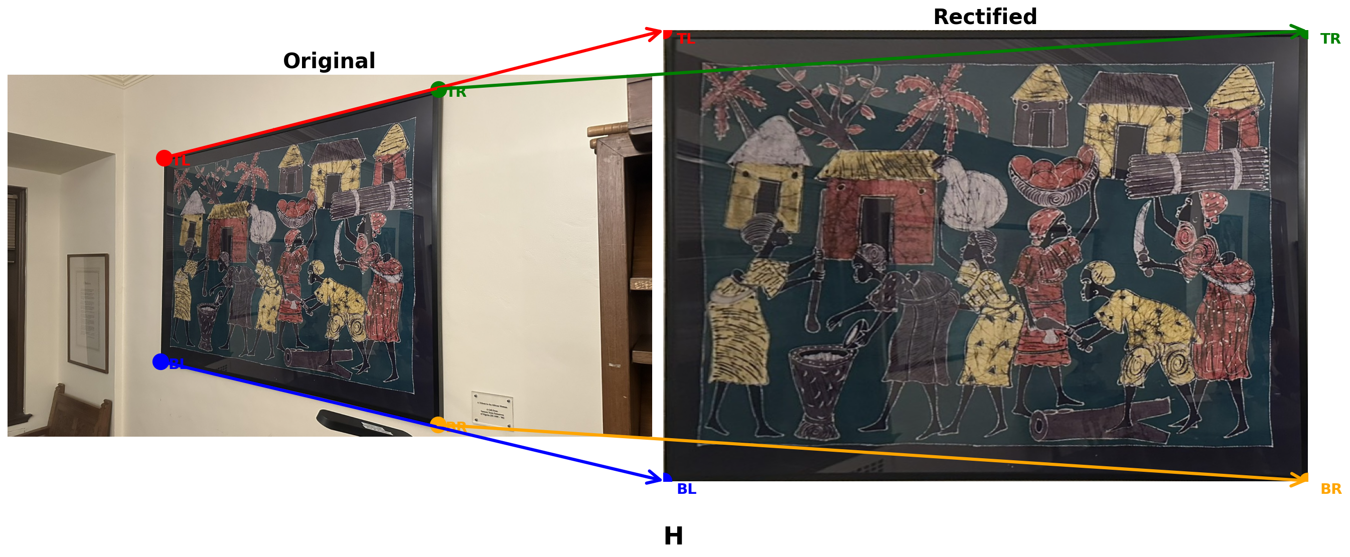
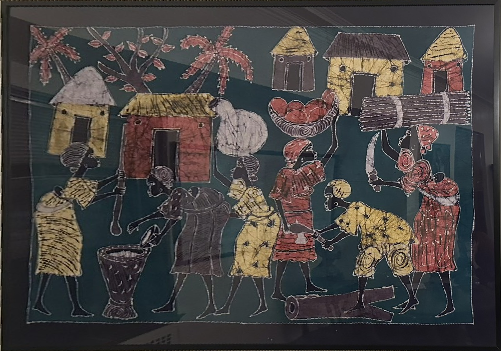
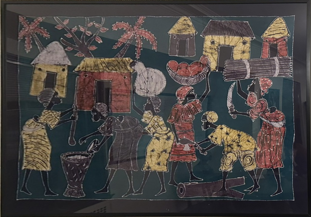
return out_h, out_w, offsetSimilar to Part A.2, we used part2_computeH and the CLI script to select the four corners of rectangular objects for rectification.
We demonstrate both interpolation methods on a sample image. Notice the difference in edge quality:
🖱️ Click to enlarge
🖱️ Click to enlarge
🖱️ Click to enlarge
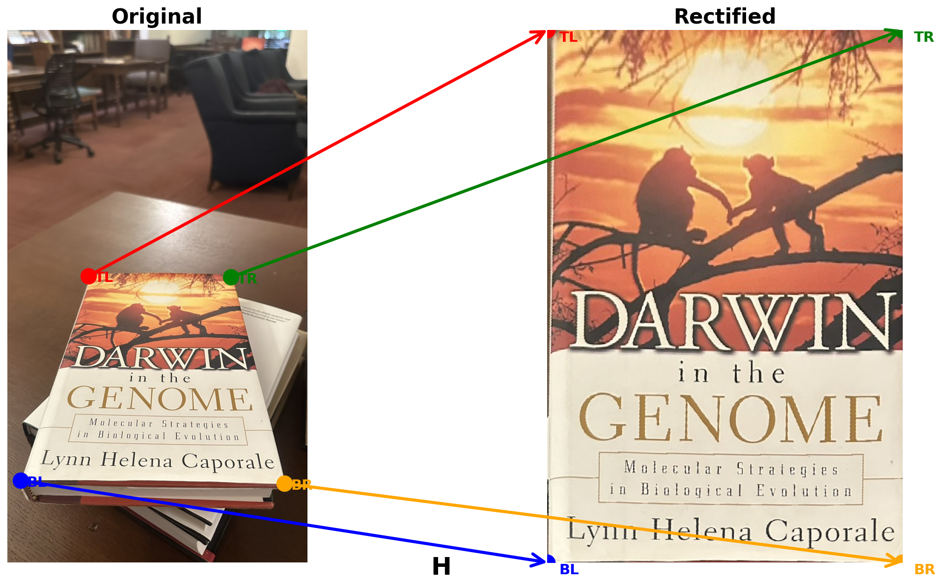
🖱️ Click to enlarge
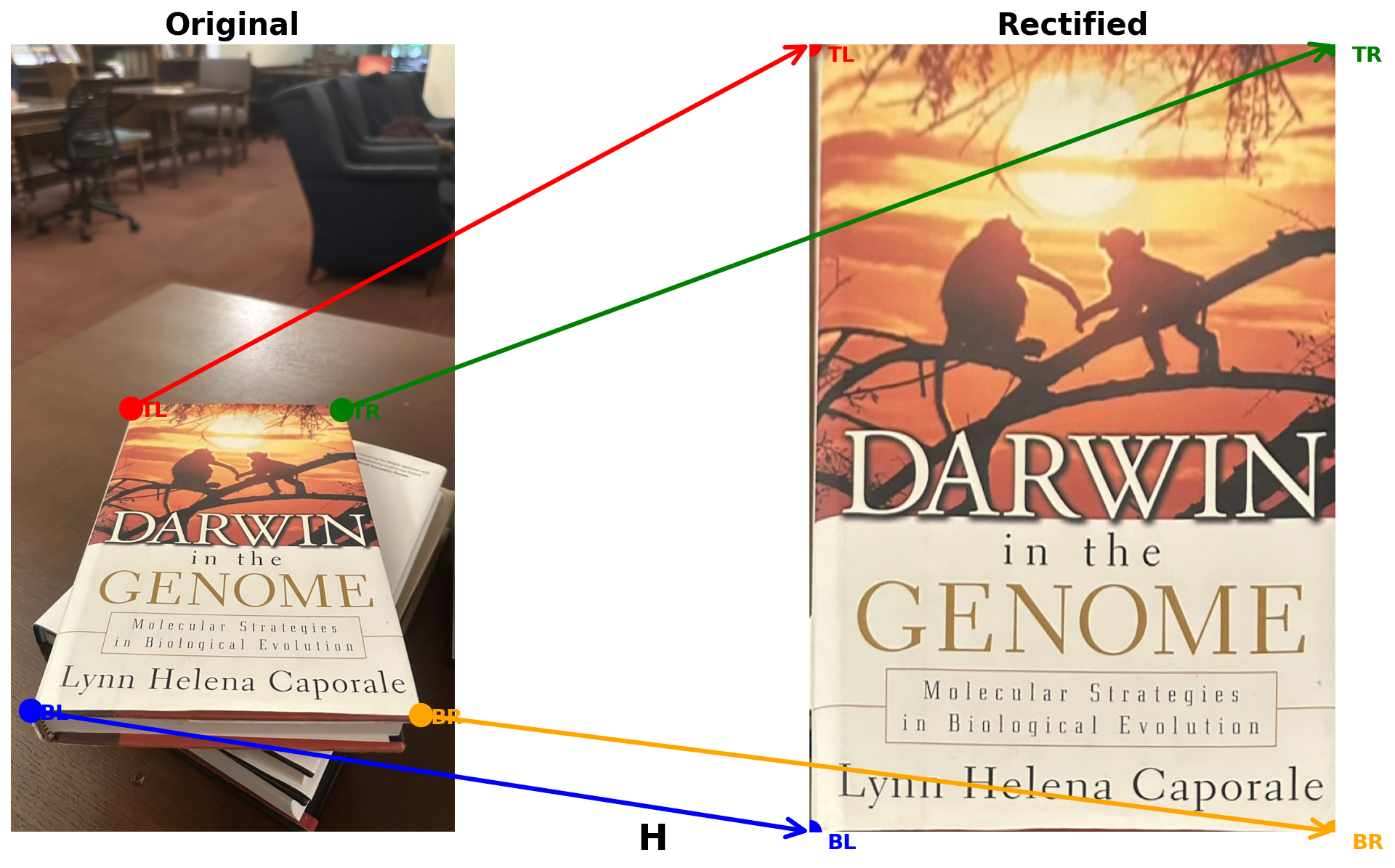
Below are rectified and cropped images from two different scenes, including nearest neighbor and bilinear interpolation methods.
After aligning all images, we implemented weighted averaging to blend them together instead of simply overlapping.
In Part A.3, we already created an alpha mask for each image to define its visible region. The alpha values are further smoothed using a distance transform, giving higher weights near the image center and gradually fading toward the edges.
create_distance_alpha
def create_distance_alpha(alpha_mask):
    """Convert binary alpha mask to distance-weighted alpha values"""
    dist = scipy.ndimage.distance_transform_edt(alpha_mask)
    max_dist = dist.max()
    if max_dist > 0:
        return dist / max_dist
return alpha_mask.astype(float)blend_images_weighted
def blend_images_weighted(images_with_alpha, use_distance_blend=True):
    """Blend multiple images using distance-weighted alpha blending"""
    ref_h, ref_w = images_with_alpha[0].shape[:2]
    has_color = len(images_with_alpha[0].shape) == 3 and images_with_alpha[0].shape[2] == 4

    if has_color:
        output = np.zeros((ref_h, ref_w, 3))
    else:
        output = np.zeros((ref_h, ref_w))

    total_weight = np.zeros((ref_h, ref_w))

    for img in images_with_alpha:
        if has_color:
            rgb = img[..., :3]
            alpha = img[..., 3]
        else:
            rgb = img[..., 0]
            alpha = img[..., 1]

        # Apply distance-based weighting
        if use_distance_blend:
            alpha = create_distance_alpha(alpha > 0) * alpha

        output += rgb * alpha[..., np.newaxis] if has_color else rgb * alpha
        total_weight += alpha

    # Normalize by total weight
    valid = total_weight > 0
    if has_color:
        output[valid] /= total_weight[valid, np.newaxis]
    else:
        output[valid] /= total_weight[valid]

return outputcreate_mosaic
def create_mosaic(images, H_list, ref_idx=0, use_distance_blend=True):
    """Create a mosaic from multiple images with computed homographies"""
    # Compute the bounding box for all warped images
    mosaic_h, mosaic_w, offset = compute_mosaic_bounds(images, H_list, ref_idx)

    # Adjust homographies to account for offset
    T_offset = np.array([[1, 0, -offset[0]], [0, 1, -offset[1]], [0, 0, 1]])

    warped_images = []

    # Warp each image to the common reference frame
    for i, im in enumerate(images):
        if i == ref_idx:
            H_adjusted = T_offset
        else:
            H_adjusted = T_offset @ H_list[i]

        warped = warpImageBilinear(im, H_adjusted, (mosaic_h, mosaic_w))
        warped_images.append(warped)

    # Blend all warped images
    mosaic = blend_images_weighted(warped_images, use_distance_blend)

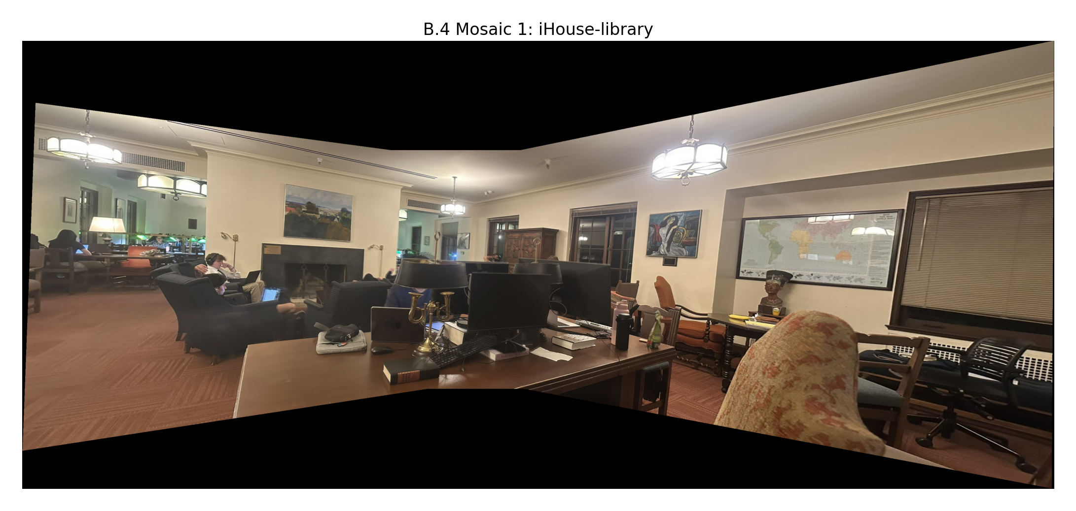
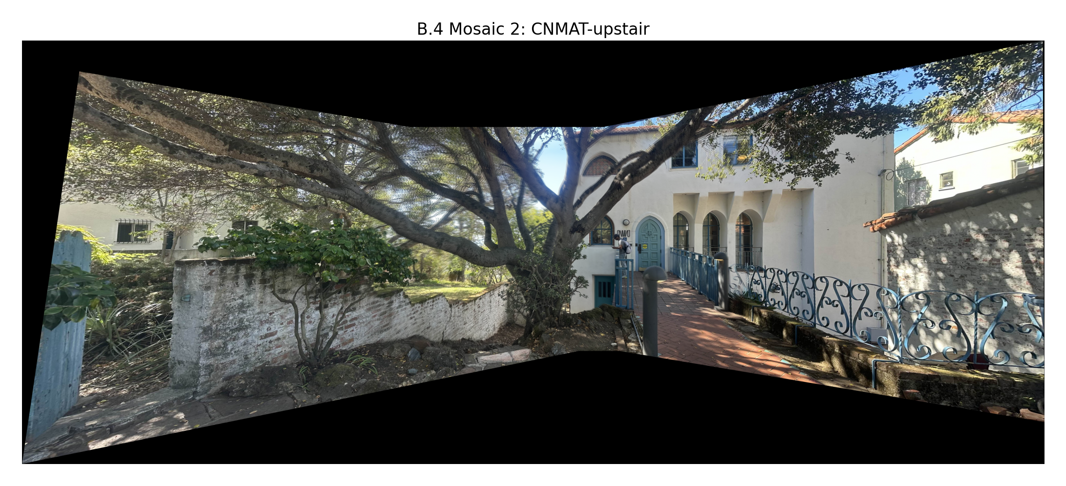
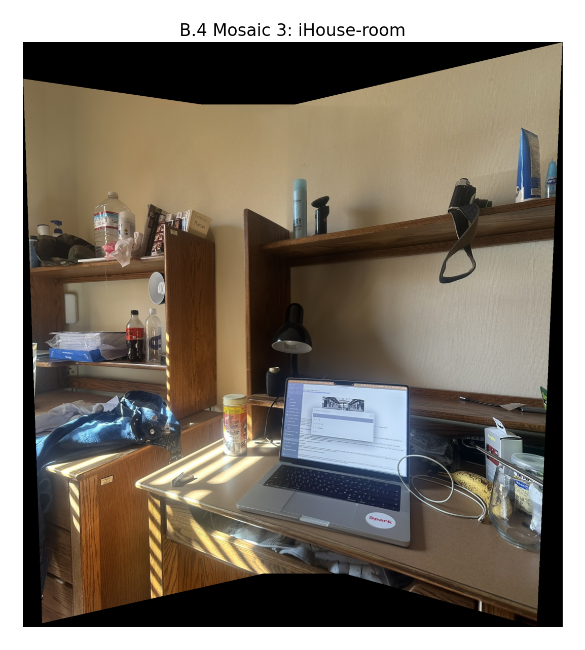
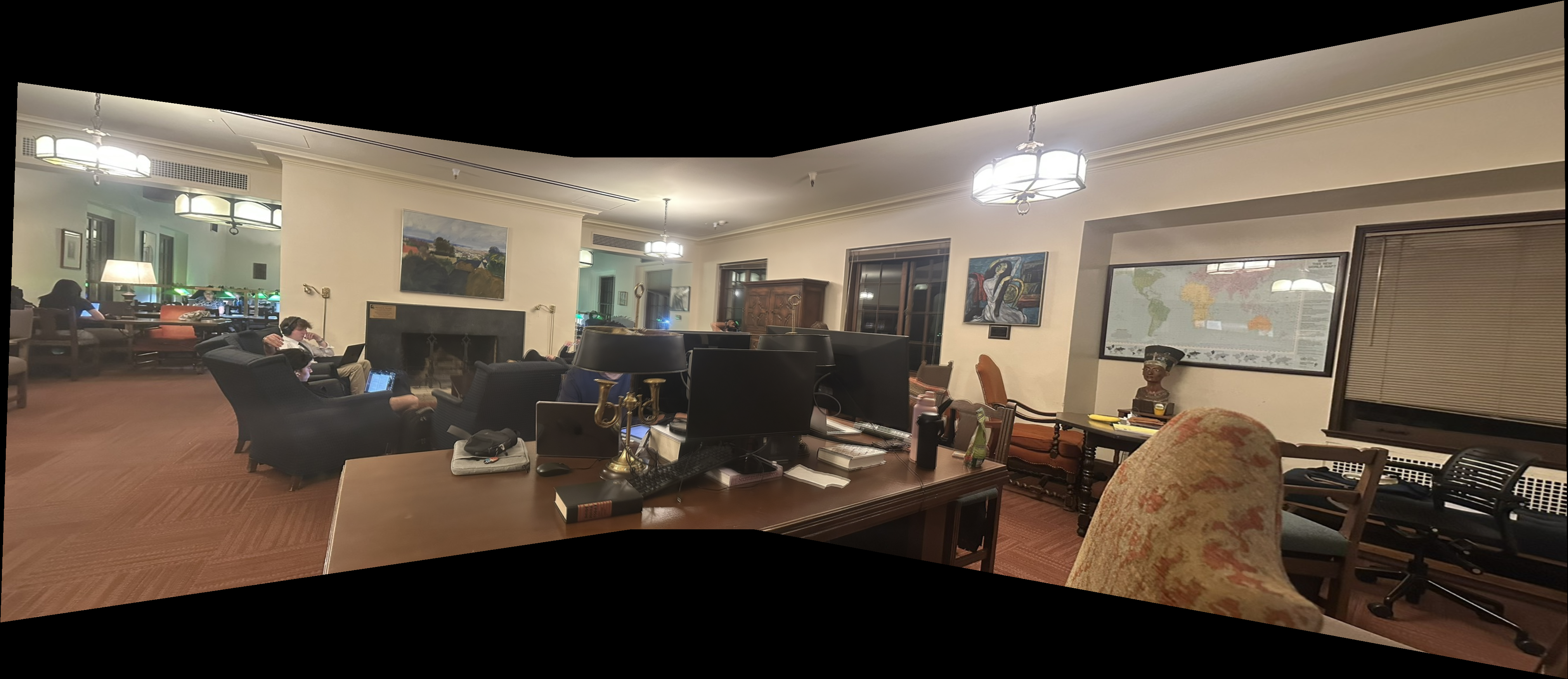
return mosaic, offsetcompute_mosaic_bounds() — Warps all image corners to find the bounding box of the final mosaicBelow are the final panoramic mosaics created by blending three images from each scene. The distance-weighted alpha blending creates seamless transitions in overlapping regions.
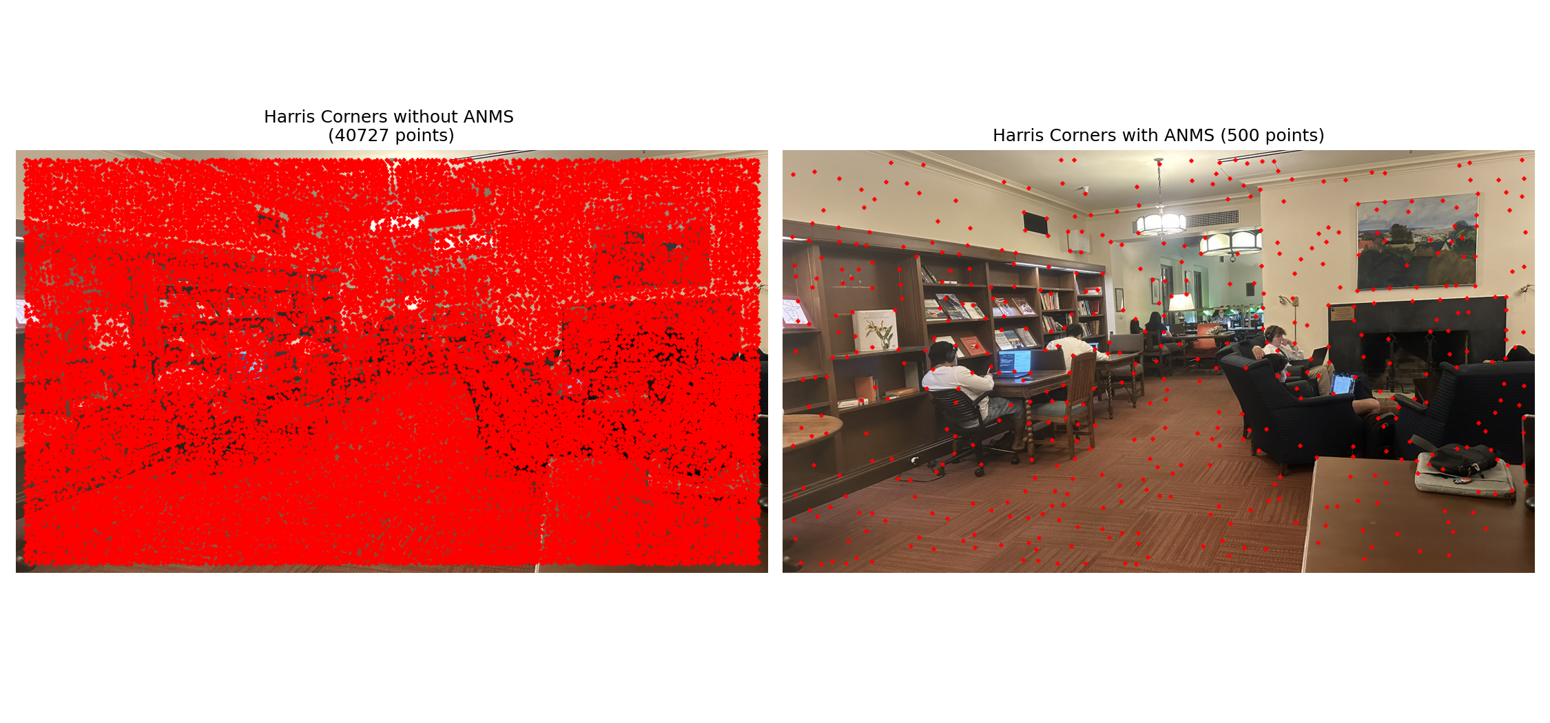
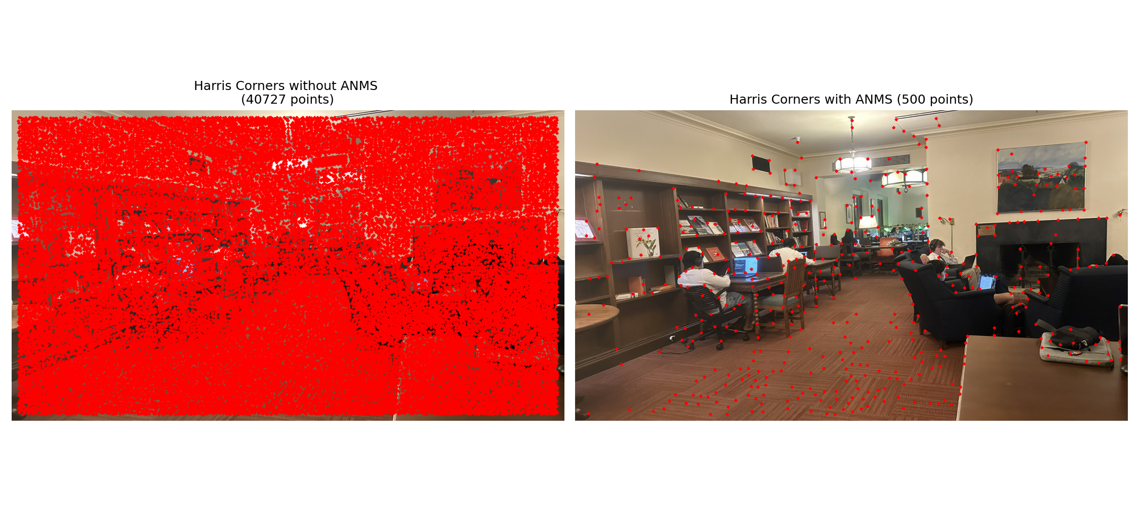
Automatic feature detection using Harris corners and Adaptive Non-Maximal Suppression (ANMS) to identify distinctive points for matching.
For each pixel, we compute the structure tensor matrix M using image gradients:
∑I²ₓ ∑IₓIᵧ∑IₓIᵧ ∑I²ᵧThe Harris response is calculated as:
R = det(M) / trace(M)R = (M₁₁·M₂₂ - M²₁₂) / (M₁₁ + M₂₂)Corners have large positive R values, edges have near-zero values, and flat regions have small values.
ANMS ensures spatial distribution of corners by:
n points with largest minimum distancesIf a corner point has a large minimum distance to any stronger corner, it means:
We use skimage.feature.corner_harris for robustness and efficiency, with custom ANMS implementation for spatial distribution.
get_harris_corners
# from harris.py ref code
def get_harris_corners(im, edge_discard=20, min_dis=1, threshold=None):
    """
    This function takes a b&w image and an optional amount to discard
    on the edge (default is 5 pixels), and finds all harris corners
    in the image. Harris corners near the edge are discarded and the
    coordinates of the remaining corners are returned. A 2d array (h)
    containing the h value of every pixel is also returned.

    h is the same shape as the original image, im.
    coords is 2 x n (ys, xs).
    """
    assert edge_discard >= 20

    # find harris corners
    h = corner_harris(im, method='eps', sigma=1)
    coords = peak_local_max(h, min_distance=min_dis, threshold_rel=threshold)

    # discard points on edge
    edge = edge_discard  # pixels
    mask = (coords[:, 0] > edge) & \
           (coords[:, 0] < im.shape[0] - edge) & \
           (coords[:, 1] > edge) & \
           (coords[:, 1] < im.shape[1] - edge)
    coords = coords[mask].T
return h, coordsanms
def anms(h, coords, c=0.9, max_pts=500):
    """
    Adaptive Non-Maximal Suppression
    Select spatially distributed corners based on their response values
    """
    if coords.shape[1] <= max_pts:
        return coords

    h_vals = h[coords[0], coords[1]]
    n = coords.shape[1]

    coords_t = coords.T
    dists = dist2(coords_t, coords_t)

    r = np.zeros(n)
    for i in range(n):
        # Find points with stronger response than c * current point
        stronger = h_vals > c * h_vals[i]
        stronger[i] = False  # Exclude self

        if np.any(stronger):
            r[i] = np.min(dists[i, stronger])
        else:
            r[i] = np.inf

    # Handle infinite values
    r[r == np.inf] = np.max(r[r != np.inf]) + 1 if np.any(r != np.inf) else 0

    # Select top max_pts points with largest minimum distances
    selected = np.argpartition(-r, max_pts)[:max_pts]

return coords[:, selected]dist2
def dist2(x, c):
    """
    Calculates squared distance between two sets of points.
    Returns M x L matrix where entry (i,j) is squared distance
    from point i in x to point j in c.
    """
    ndata, dimx = x.shape
    ncenters, dimc = c.shape
    assert dimx == dimc, 'Data dimension does not match dimension of centers'

    return (np.ones((ncenters, 1)) * np.sum((x**2).T, axis=0)).T + \
            np.ones((ndata, 1)) * np.sum((c**2).T, axis=0) - \
2 * np.inner(x, c)We can significantly improve performance by pre-filtering corners using peak_local_max parameters:
threshold_rel — Filters out weak corners below relative thresholdmin_distance — Ensures minimum spacing between detected cornersThis pre-filtering removes noise points and reduces ANMS computation time from 3m 29.9s to just 0.4s for n=500 points.
Comparing Harris corner detection with and without pre-filtering optimization on the same scene.
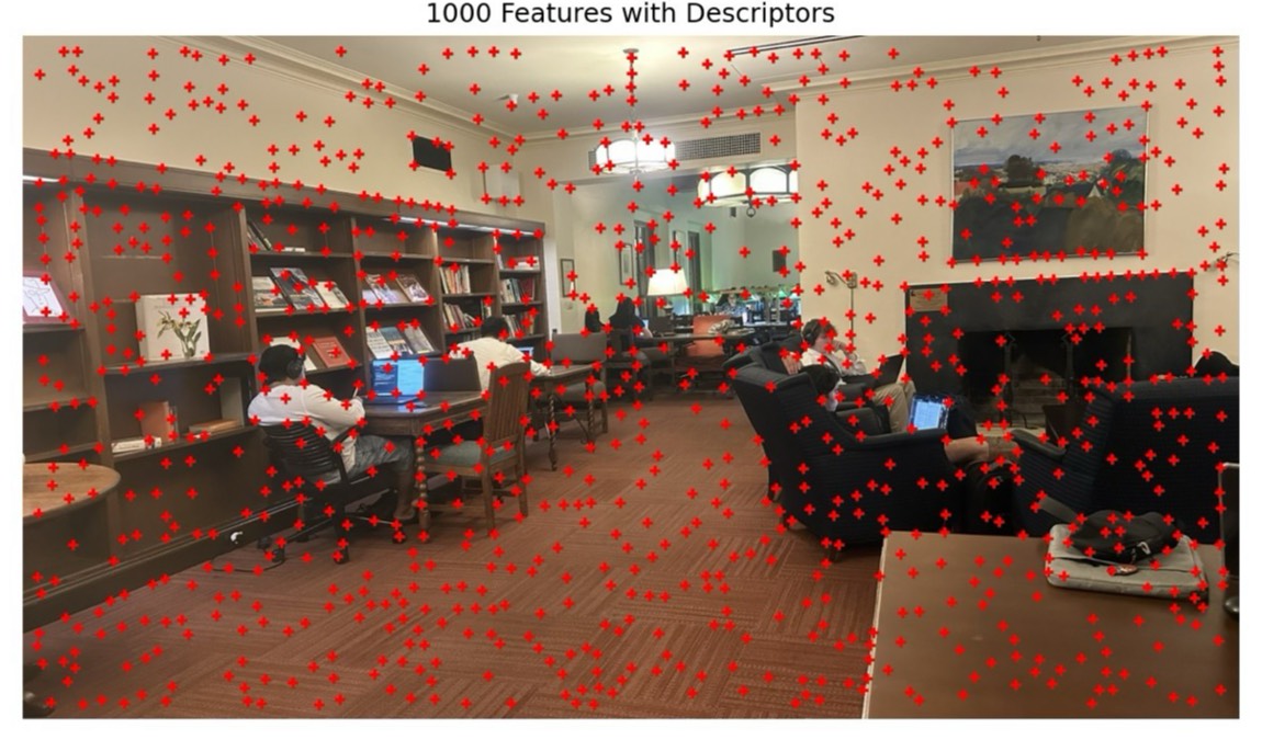
Based on Section 4 of the MOPS paper, we extract descriptors using a multi-scale approach:
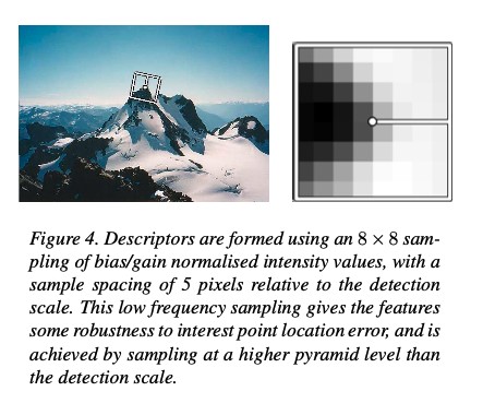
extract_feature_descriptors
def extract_feature_descriptors(im, coords):
    """
    Extract MOPS-style feature descriptors from detected corners.
    Returns 64-dimensional normalized descriptors for each valid corner.
    """
    h, w = im.shape
    blurred = gaussian_filter(im, sigma=1.5)

    descriptors = []
    valid_coords = []

    for i in range(coords.shape[1]):
        y, x = coords[0, i], coords[1, i]

        # Check if 40x40 window fits within image bounds
        if 20 <= y < h-20 and 20 <= x < w-20:
            # Extract 40x40 window centered at corner
            window = blurred[y-20:y+20, x-20:x+20]

            # Downsample by factor of 5 to get 8x8 descriptor
            descriptor = window[::5, ::5][:8, :8].flatten()

            # Normalize descriptor to zero mean and unit variance
            mean, std = descriptor.mean(), descriptor.std()
            descriptor = (descriptor - mean) / std if std > 0 else descriptor - mean

            descriptors.append(descriptor)
            valid_coords.append([y, x])

return np.array(descriptors), np.array(valid_coords).TFor demonstration purposes, we deliberately used relaxed parameters to show both good and bad descriptors: min_dis=3, threshold=None, max_pts=32.
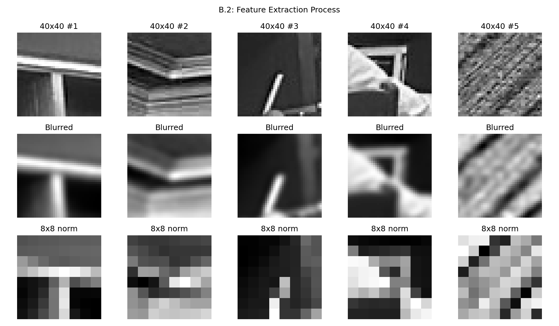
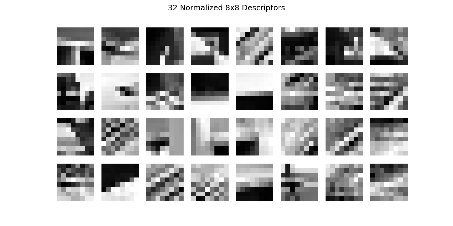
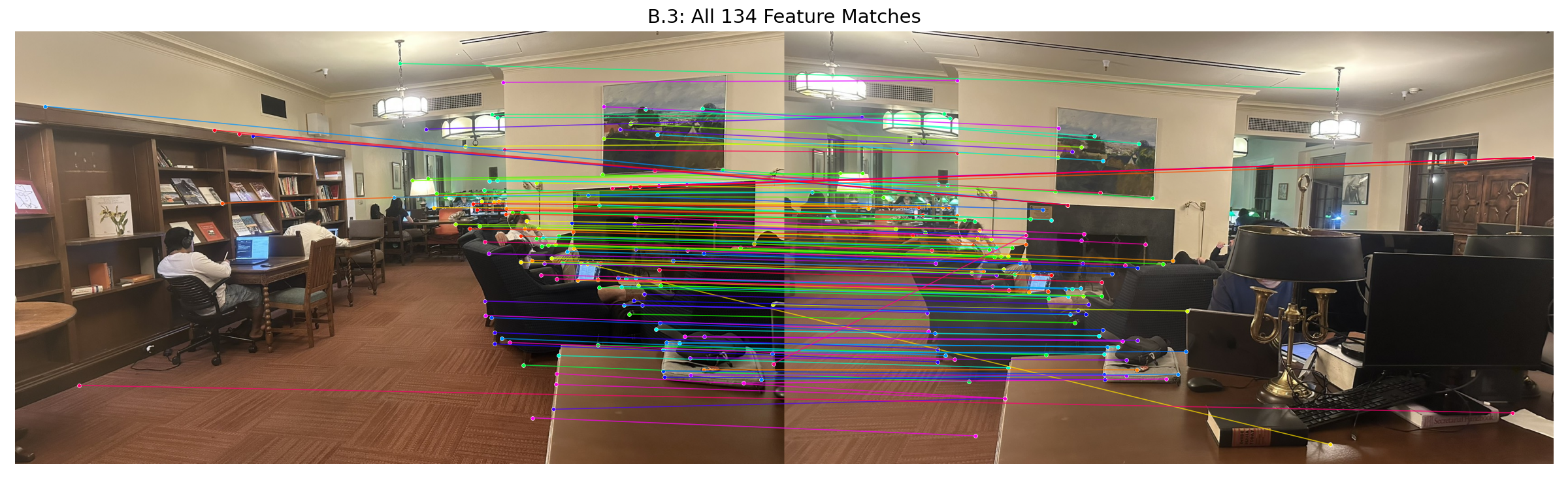
Our goal is to find pairs of features that look similar and are thus likely to be good matches between two images.
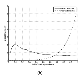
To distinguish reliable matches from ambiguous ones, we use the ratio test proposed by David Lowe:
r = dist(1st NN) / dist(2nd NN)r < threshold, accept it as a good matchAccording to Figure 6(b) from the MOPS paper, we can observe the distribution of matching errors for correct and incorrect matches. The ratio of 1-NN / 2-NN provides a good metric for distinguishing matches:
match_features
# Lowe's ratio test
def match_features(descriptors1, descriptors2, ratio_threshold=0.7):
    """
    Match features using Lowe's ratio test.
    For each feature in descriptors1, find the best and second-best matches
    in descriptors2. Accept the match if the ratio of distances is below threshold.
    """
    if len(descriptors1) == 0 or len(descriptors2) == 0:
        return np.array([]).reshape(0, 2)

    # Compute all pairwise distances
    distances = np.sqrt(dist2(descriptors1, descriptors2))
    matches = []

    for i in range(len(descriptors1)):
        # Find two nearest neighbors
        sorted_indices = np.argsort(distances[i])

        if len(sorted_indices) >= 2:
            # Ratio test: first/second nearest neighbor
            ratio = distances[i, sorted_indices[0]] / distances[i, sorted_indices[1]]

            if ratio < ratio_threshold:
                matches.append([i, sorted_indices[0]])

return np.array(matches) if matches else np.array([]).reshape(0, 2)Below we show the matched features between two images from the IHouse Library scene using different visualization approaches.
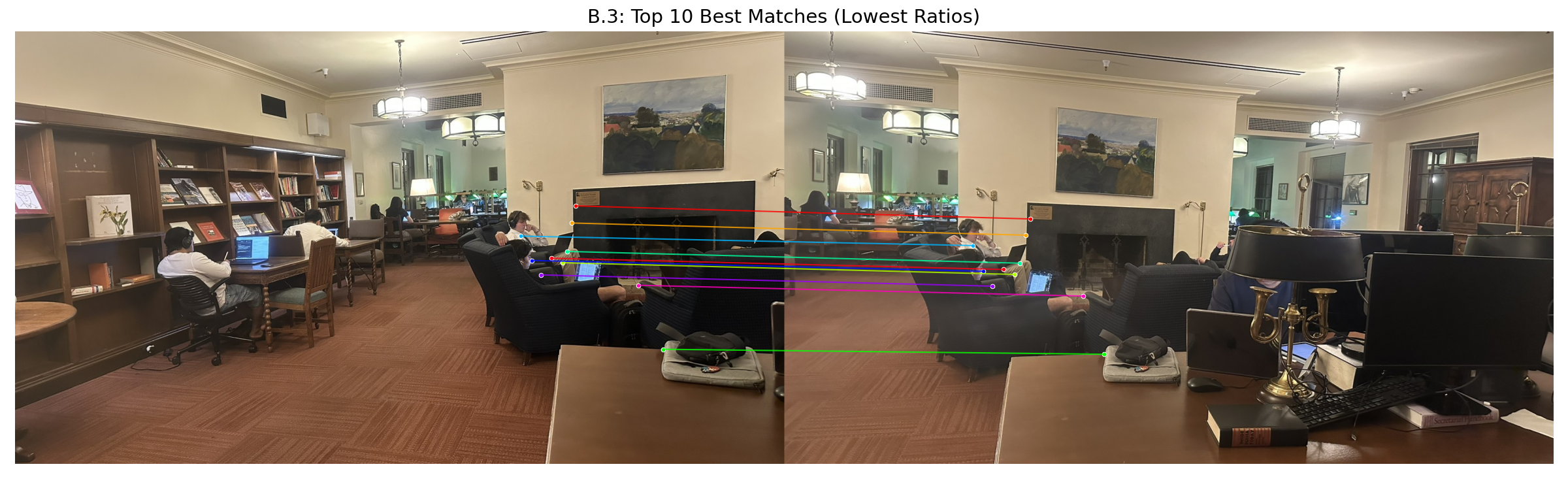
Even with Lowe's ratio test, some incorrect matches may remain. RANSAC iteratively finds the homography that best fits the largest subset of matches.
The algorithm repeatedly samples small subsets of matches to find the best homography:
RANSAC reuses the computeH() function from Part A.2 to compute homographies from point correspondences.
error = ||H·p₁ - p₂||
Points with error < threshold are classified as inliers
ransac_homography
def ransac_homography(matches, coords1, coords2, n_iters=5000, threshold=3.0):
    """
    Robustly estimate homography using RANSAC.
    Returns the best homography and a boolean mask of inliers.
    """
    if len(matches) < 4:
        return None, np.zeros(len(matches), dtype=bool)

    # Convert (y,x) to (x,y) for computeH
    pts1 = np.array([[coords1[1, m[0]], coords1[0, m[0]]] for m in matches])
    pts2 = np.array([[coords2[1, m[1]], coords2[0, m[1]]] for m in matches])

    best_H = None
    best_inliers = np.zeros(len(matches), dtype=bool)
    max_inliers = 0


    for _ in range(n_iters):
        # 1. Randomly sample 4 matches
        idx = np.random.choice(len(matches), 4, replace=False)

        # 2. Compute homography using Part A.2's computeH
        H, _, _ = computeH(pts1[idx], pts2[idx])

        # 3. Compute reprojection errors
        pt1_h = np.column_stack([pts1, np.ones(len(pts1))])
        pt2_proj = (H @ pt1_h.T).T
        pt2_proj = pt2_proj[:, :2] / pt2_proj[:, 2:]
        errors = np.linalg.norm(pt2_proj - pts2, axis=1)

        # 3. Count inliers
        inliers = errors < threshold

        # 4. Keep the best H
        if np.sum(inliers) > max_inliers:
            max_inliers = np.sum(inliers)
            best_inliers = inliers
            best_H = H

        # 5. Loop back to step 1

    # Refine with all inliers
    if max_inliers >= 4:
        best_H, _, _ = computeH(pts1[best_inliers], pts2[best_inliers])

    print(f"  RANSAC: {max_inliers}/{len(matches)} inliers")
return best_H, best_inliersstitch_images
def stitch_images(image_paths, ref_idx=None, ratio_threshold=0.7, ransac_iters=5000,
                  ransac_threshold=3.0, max_pts=1000, feather_width=150):
    """
    Fully automatic image stitching pipeline using Harris corners, MOPS descriptors,
    Lowe's ratio test, and RANSAC.
    """
    images = [sk.img_as_float(skio.imread(p)) for p in image_paths]

    if ref_idx is None:
        ref_idx = len(images) // 2

    n = len(images)
    pairwise_H = [[None] * n for _ in range(n)]

    for i in range(n - 1):
        im1_gray = sk.color.rgb2gray(images[i]) if len(images[i].shape) == 3 else images[i]
        im2_gray = sk.color.rgb2gray(images[i+1]) if len(images[i+1].shape) == 3 else images[i+1]

        # B.1 Detect Harris corners
        h1, coords1 = get_harris_corners(im1_gray, edge_discard=20, min_dis=10, threshold=0.01)
        h2, coords2 = get_harris_corners(im2_gray, edge_discard=20, min_dis=10, threshold=0.01)

        # B.2 Apply ANMS
        coords1_anms = anms(h1, coords1, max_pts=max_pts)
        coords2_anms = anms(h2, coords2, max_pts=max_pts)

        # B.2 Extract MOPS descriptors
        descriptors1, coords1_valid = extract_feature_descriptors(im1_gray, coords1_anms)
        descriptors2, coords2_valid = extract_feature_descriptors(im2_gray, coords2_anms)

        # B.3 Match features using Lowe's ratio test
        matches, _ = match_features(descriptors1, descriptors2, ratio_threshold=ratio_threshold)
        print(f"  Matches: {len(matches)}")

        # B.4 Robustly estimate homography using RANSAC
        H, inliers = ransac_homography(matches, coords1_valid, coords2_valid,
                                      n_iters=ransac_iters, threshold=ransac_threshold)

        if H is not None:
            pairwise_H[i][i+1] = H
            pairwise_H[i+1][i] = np.linalg.inv(H)

    # Chain homographies relative to reference image
    H_list = [None] * n
    H_list[ref_idx] = np.eye(3)

    # Left side of reference
    for i in range(ref_idx - 1, -1, -1):
        if pairwise_H[i][i+1] is not None:
            H_list[i] = pairwise_H[i][i+1] @ H_list[i+1]

    # Right side of reference
    for i in range(ref_idx + 1, n):
        if pairwise_H[i][i-1] is not None:
            H_list[i] = pairwise_H[i][i-1] @ H_list[i-1]

    # Create final mosaic using Part A.4's create_mosaic
    mosaic, _ = create_mosaic(images, H_list, ref_idx, use_distance_blend=True,
                             feather_width=feather_width)

return mosaicBelow are panoramic mosaics created using the fully automatic stitching pipeline. Compare these with the manual results from Part A.4 to see the effectiveness of automatic feature matching.