Part 0.1: Camera Calibration
The goal of camera calibration is to estimate the intrinsic matrix and distortion coefficients of the camera. These parameters are essential for later stages (pose estimation and 3D reconstruction) and must remain constant throughout the entire capture process — this is why the assignment spec emphasizes not adjusting the camera's focal length/zoom.
By capturing multiple images of ArUco calibration tags from different angles and distances, we can solve for the camera's internal parameters using known 3D-to-2D correspondences.
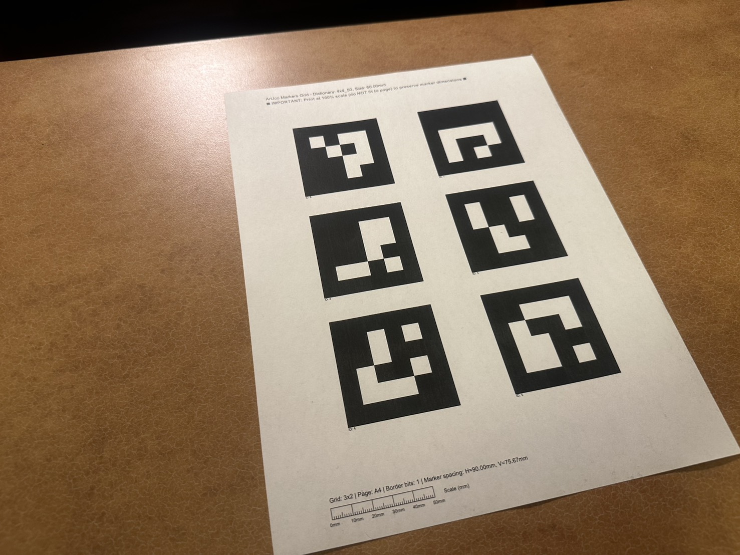
Implementation
Note: OpenCV Version Compatibility
The spec uses syntax for OpenCV < 4.7.0. My implementation uses the updated API for newer versions. See this StackOverflow discussion for details.
Camera Calibration Implementation
Camera path + novel views
def create_circular_path(base_pos, num_frames):
    radius = np.sqrt(base_pos[0]**2 + base_pos[1]**2)
    fixed_z = base_pos[2]
    c2ws = []
    for i in range(num_frames):
        angle = (i / num_frames) * 2 * np.pi
        cam_x = radius * np.cos(angle)
        cam_y = radius * np.sin(angle)
        cam_pos = np.array([cam_x, cam_y, fixed_z])

        forward = -cam_pos / np.linalg.norm(cam_pos)
        world_up = np.array([0, 0, 1])
        right = np.cross(forward, world_up); right /= np.linalg.norm(right)
        up = np.cross(right, forward); up /= np.linalg.norm(up)

        c2w = np.eye(4)
        c2w[:3, 0] = right
        c2w[:3, 1] = up
        c2w[:3, 2] = forward
        c2w[:3, 3] = cam_pos
        c2ws.append(c2w)
    return c2ws

def render_novel_views(model, data_path, num_frames, save_path,
                       n_samples, near, far, device, white_bkgd=True):
    data = np.load(data_path)
    c2ws_train = data['c2ws_train']
    K = data['K'] if 'K' in data else np.array([
        [data['focal'], 0, data['images_train'].shape[2] / 2],
        [0, data['focal'], data['images_train'].shape[1] / 2],
        [0, 0, 1]
    ])
    H, W = data['images_train'].shape[1:3]

    c2ws = create_circular_path(c2ws_train[0, :3, 3], num_frames)
    eval_model = model.module if hasattr(model, 'module') else model
    eval_model.eval()

    frames = []
    with torch.no_grad():
        for c2w in c2ws:
            frame = render_image(eval_model,
                                 torch.FloatTensor(c2w),
                                 H, W, K,
                                 n_samples=n_samples,
                                 near=near, far=far,
                                 device=device)
            frames.append((np.clip(frame, 0, 1) * 255).astype(np.uint8))

    pil_frames = [Image.fromarray(f) for f in frames]
    pil_frames[0].save(save_path, save_all=True,
                       append_images=pil_frames[1:],
                       duration=33, loop=0)
Results
Images processed: 33/33 images (100% detection rate)
Total tag detections: 198 tags
Reprojection Error: 0.786 pixels
Camera Intrinsic Matrix (K):
[[957.34    0.00  795.40]
 [  0.00  949.21  594.72]
 [  0.00    0.00    1.00]]
Distortion Coefficients: [k₁, k₂, p₁, p₂, k₃]
[0.261, -1.723, 0.018, 0.027, 2.748]
Part 0.2: Capturing a 3D Object Scan
I placed my Miffy doll next to the calibration tag and shot 38 photos while orbiting the bunny, keeping exposure/focus fixed so the poses stay consistent. The raw captures live at images/0-miffy-two/. (Fun fact: I first tried the CalHacks 12.0 bear, but the busy background made training unstable, so I re-shot with Miffy—Part 1 still uses the bear!)
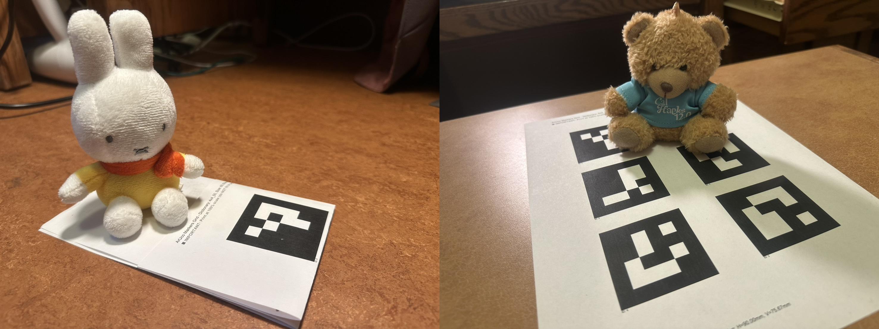
Before training Part 2, I resize the photos down to 373×280 so they match the intrinsics of the provided Lego dataset. A tiny Pillow script batches the conversion:
Batch resizing script
import os
from PIL import Image

input_folder = "images/0-miffy-two"
output_folder = "images/0-miffy-two-resize"
target_size = (373, 280)

os.makedirs(output_folder, exist_ok=True)

for filename in os.listdir(input_folder):
    if filename.lower().endswith((".jpg", ".jpeg", ".png")):
        img_path = os.path.join(input_folder, filename)
        img = Image.open(img_path)
        img_resized = img.resize(target_size, Image.LANCZOS)
        img_resized.save(os.path.join(output_folder, filename))
        print(f"Done: {filename}")

print("All images resized!")
The resized set in images/0-miffy-two-resize/ becomes the dataset I feed into the NeRF dataloader later on.
Part 0.3: Camera Pose Estimation
The goal of this step is to estimate the extrinsic parameters (rotation and translation) for each camera pose. This is known as the Perspective-n-Point (PnP) problem: given a set of 3D points in world coordinates and their corresponding 2D projections in an image, we solve for the camera's position and orientation in 3D space.
Implementation
Important: World-to-Camera vs Camera-to-World
solvePnP() returns the world-to-camera (w2c) transformation.For NeRF, we need the camera-to-world (c2w) transformation, so we must invert the result:
c2w = [R | t] = [R₀₀  R₀₁  R₀₂  tₓ]
      [0 | 1]   [R₁₀  R₁₁  R₁₂  tᵧ]
                [R₂₀  R₂₁  R₂₂  t_z]
                [ 0    0    0    1 ]
Pose Estimation Implementation
Visualization with Viser
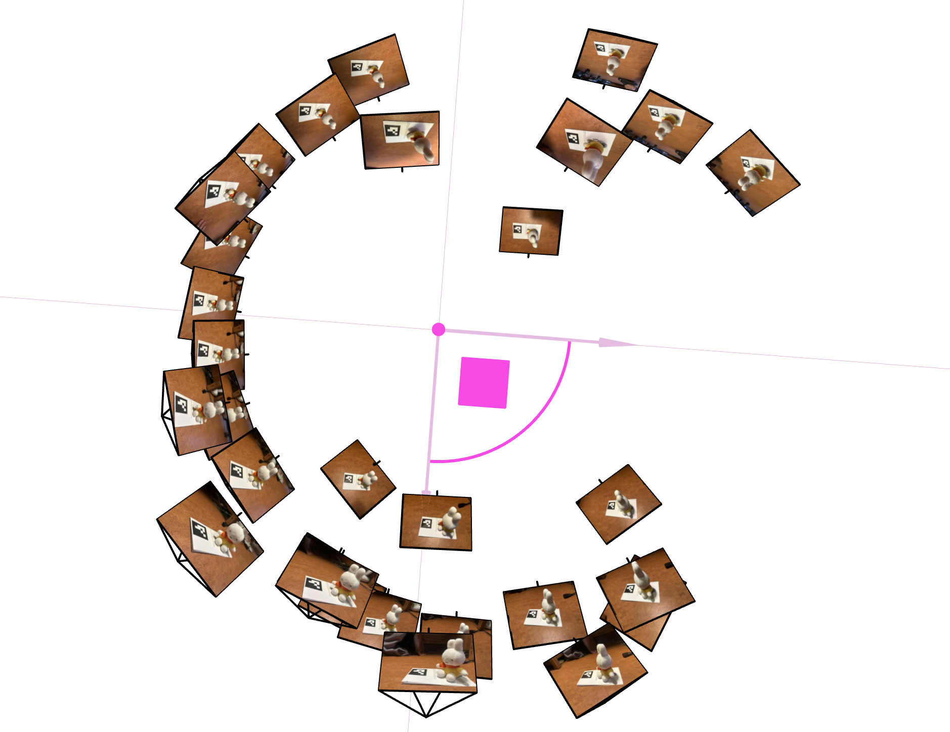
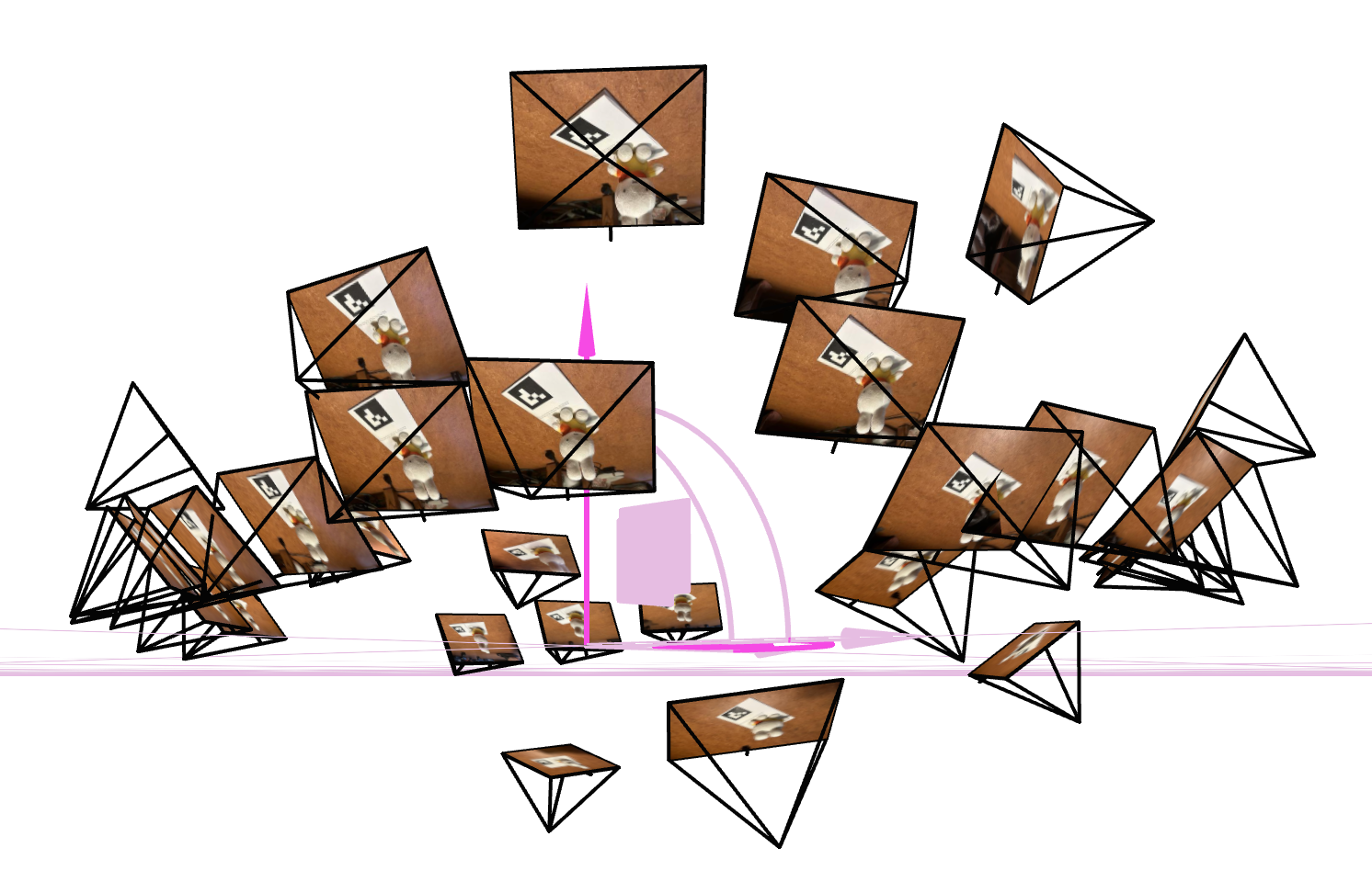
To verify our pose estimation, we visualize all camera frustums in 3D space using viser.
3D Frustum Visualization
Results
Part 0.4: Dataset Preparation
The final step is to undistort all images and package everything into a dataset format ready for NeRF training. This combines all previous steps from Part 0.1 to 0.3.
Implementation
Dataset Creation Implementation
Dataset Structure
Output: my_data.npz
The packaged dataset contains:
images_train: Training images (undistorted RGB)c2ws_train: Camera-to-world matrices for training (0.7)images_val: Validation imagesc2ws_val: Camera-to-world matrices for validation (0.15)c2ws_test: Camera-to-world matrices for test (0.15)K: Full intrinsic matrix (switched from scalar focal because it made Part 2.6 result better)
Part 1: Neural Field for 2D Images
Before jumping into 3D NeRF, which learns the mapping F: {x, y, z, θ, φ} → {r, g, b, σ}, we start with 2D as a simpler introduction. In 2D, we only need to solve F: {u, v} → {r, g, b}, where {u, v} represents 2D pixel coordinates.
1.1 Sinusoidal Positional Encoding (PE)
Positional encoding helps neural networks capture high-frequency details by transforming input coordinates into a higher-dimensional space using sinusoidal functions. Without PE, MLPs struggle to represent fine details in images.
The encoding applies sine and cosine functions at different frequencies:

Positional Encoding Implementation
class PositionalEncoding(nn.Module):
    def __init__(self, L=10):
        super().__init__()
        self.L = L

    def forward(self, x):
        out = [x]
        for i in range(self.L):
            out.append(torch.sin(2**i * np.pi * x))
            out.append(torch.cos(2**i * np.pi * x))
        return torch.cat(out, dim=-1)
For L=10 frequency bands, a 2D coordinate is transformed from dimension 2 to dimension 2 + 2×L×2 = 42.
1.2 Multilayer Perceptron (MLP) Architecture
Our neural field network follows the architecture shown below:
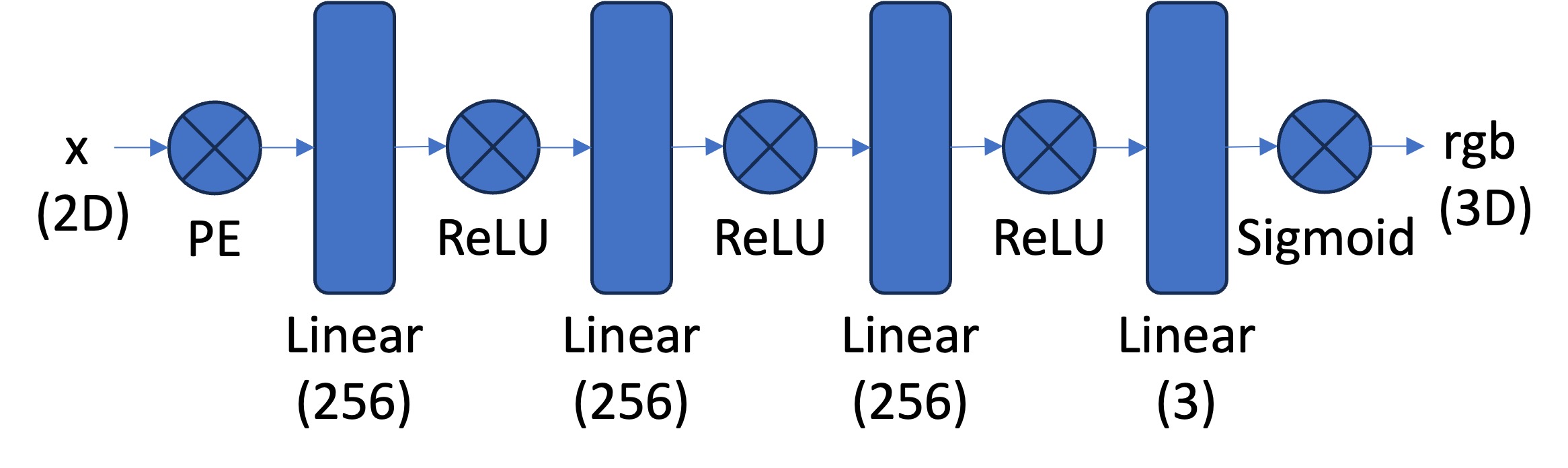
The network consists of:
- Input: 2D pixel coordinates (u, v)
- Positional Encoding: Expands input to 42 dimensions
- Hidden Layers: 3 fully-connected layers with 256 units each, using ReLU activation
- Output Layer: Maps to RGB values (3 channels) with Sigmoid activation to ensure [0,1] range
Neural Field 2D Implementation
class NeuralField2D(nn.Module):
    def __init__(self, L=10, hidden_dim=256):
        super().__init__()
        self.pe = PositionalEncoding(L)
        pe_dim = 2 + 2 * L * 2  # 42 dimensions

        self.mlp = nn.Sequential(
            nn.Linear(pe_dim, hidden_dim),
            nn.ReLU(),
            nn.Linear(hidden_dim, hidden_dim),
            nn.ReLU(),
            nn.Linear(hidden_dim, hidden_dim),
            nn.ReLU(),
            nn.Linear(hidden_dim, 3),
            nn.Sigmoid()
        )

    def forward(self, coords):
        encoded = self.pe(coords)
        return self.mlp(encoded)
1.3 Pixel Dataloader
Since high-resolution images are memory-intensive, we implement a dataloader that randomly samples N pixels at every iteration for training. This approach:
- Returns
N×2normalized 2D coordinates in [0,1] - Returns corresponding
N×3RGB color values in [0,1] - Enables efficient mini-batch training without loading entire images
Pixel Dataloader Implementation
class PixelDataloader:
    def __init__(self, img, batch_size=10000):
        self.img = img / 255.0  # Normalize to [0,1]
        self.H, self.W = img.shape[:2]
        self.batch_size = batch_size

        # Create normalized coordinate grid
        y, x = np.meshgrid(np.arange(self.H), np.arange(self.W), indexing='ij')
        self.coords = np.stack([x / self.W, y / self.H], axis=-1).reshape(-1, 2)
        self.colors = self.img.reshape(-1, 3)

    def sample(self):
        """Randomly sample batch_size pixels"""
        idx = np.random.choice(len(self.coords), self.batch_size, replace=False)
        coords = torch.FloatTensor(self.coords[idx])
        colors = torch.FloatTensor(self.colors[idx])
        return coords, colors

    def get_all(self):
        """Get all pixels (for validation/visualization)"""
        coords = torch.FloatTensor(self.coords)
        colors = torch.FloatTensor(self.colors)
        return coords, colors
1.4 Training: Loss Function, Optimizer, and Metric
We train the neural field to minimize the difference between predicted and ground truth pixel colors using:
- Loss Function: Mean Squared Error (MSE) between predicted and actual RGB values
- Metric: Peak Signal-to-Noise Ratio (PSNR) =
10 × log₁₀(1/MSE) - Optimizer: Adam with learning rate
1e-2 - Training: 1000-3000 iterations with batch size of 10,000 pixels
Training Loop Implementation
def train_neural_field(img_path, L=10, hidden_dim=256, lr=1e-2, iters=3000, batch_size=10000, save_dir='images'):
    os.makedirs(save_dir, exist_ok=True)

    device = torch.device('cuda' if torch.cuda.is_available() else 'mps' if torch.backends.mps.is_available() else 'cpu')
    print(f'Using device: {device}')

    img = skio.imread(img_path)
    if img.ndim == 2:
        img = np.stack([img] * 3, axis=-1)

    H, W = img.shape[:2]

    model = NeuralField2D(L=L, hidden_dim=hidden_dim).to(device)
    dataloader = PixelDataloader(img, N=batch_size)
    optimizer = torch.optim.Adam(model.parameters(), lr=lr)
    criterion = nn.MSELoss()

    psnr_history = []
    save_iters = [0, 100, 500, 1000, 2000, iters-1]

    for it in range(iters):
        coords, colors = dataloader.sample()
        coords, colors = coords.to(device), colors.to(device)

        pred_colors = model(coords)
        loss = criterion(pred_colors, colors)

        optimizer.zero_grad()
        loss.backward()
        optimizer.step()

        psnr = psnr_from_mse(loss)
        psnr_history.append(psnr.item())

        if it % 100 == 0 or it == iters - 1:
            print(f'Iter {it:4d}: Loss={loss.item():.6f}, PSNR={psnr.item():.2f} dB')

        # Save visualization at key iterations
        if it in save_iters:
            with torch.no_grad():
                y, x = np.meshgrid(np.arange(H), np.arange(W), indexing='ij')
                test_coords = np.stack([x / W, y / H], axis=-1).reshape(-1, 2)
                test_coords = torch.FloatTensor(test_coords).to(device)

                pred = []
                for i in range(0, len(test_coords), batch_size):
                    pred.append(model(test_coords[i:i+batch_size]).cpu())
                pred = torch.cat(pred, dim=0)

                pred_img = pred.reshape(H, W, 3).numpy()

                # Save comparison: GT, Prediction, Error
                plt.figure(figsize=(12, 4))
                plt.subplot(1, 3, 1)
                plt.imshow(img / 255.0)
                plt.title('Ground Truth')
                plt.axis('off')

                plt.subplot(1, 3, 2)
                plt.imshow(pred_img)
                plt.title(f'Prediction (iter {it})')
                plt.axis('off')

                plt.subplot(1, 3, 3)
                plt.imshow(np.abs(img / 255.0 - pred_img))
                plt.title('Error')
                plt.axis('off')

                plt.tight_layout()
                plt.savefig(f'{save_dir}/iter_{it:04d}.png', bbox_inches='tight', dpi=150)
                plt.close()

    # Save PSNR curve
    plt.figure(figsize=(10, 6))
    plt.plot(psnr_history)
    plt.xlabel('Iteration')
    plt.ylabel('PSNR (dB)')
    plt.title('Training PSNR')
    plt.grid(True)
    plt.savefig(f'{save_dir}/psnr_curve.png', bbox_inches='tight', dpi=150)
    plt.close()

    return model, psnr_history
1.5 Results and Analysis
1) Model Architecture
- Positional Encoding: L = 10 frequency bands (input dimension: 42)
- Network Depth: 3 hidden layers
- Layer Width: 256 units per hidden layer
- Activation: ReLU (hidden layers), Sigmoid (output layer)
- Learning Rate: 1e-2 (Adam optimizer)
- Batch Size: 10,000 pixels per iteration
- Training Iterations: 3,000
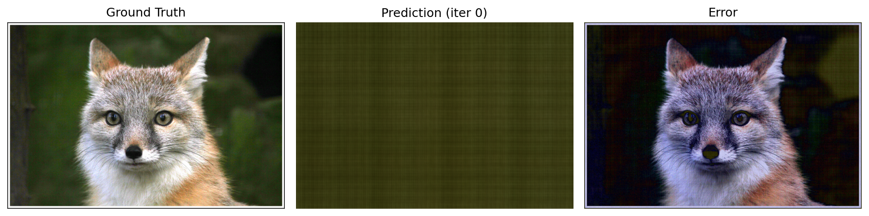
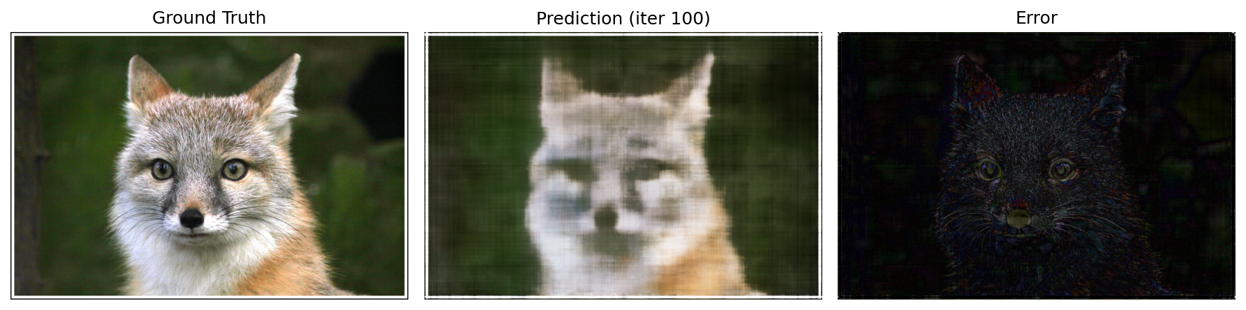
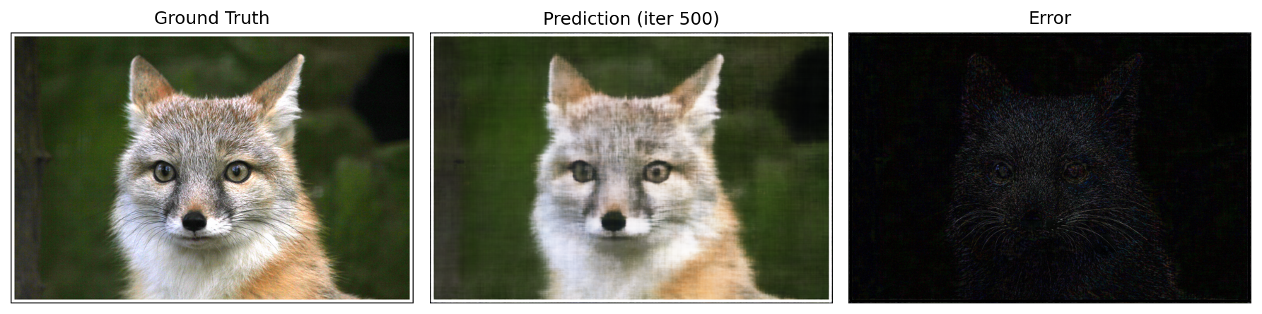
2) Training Progression
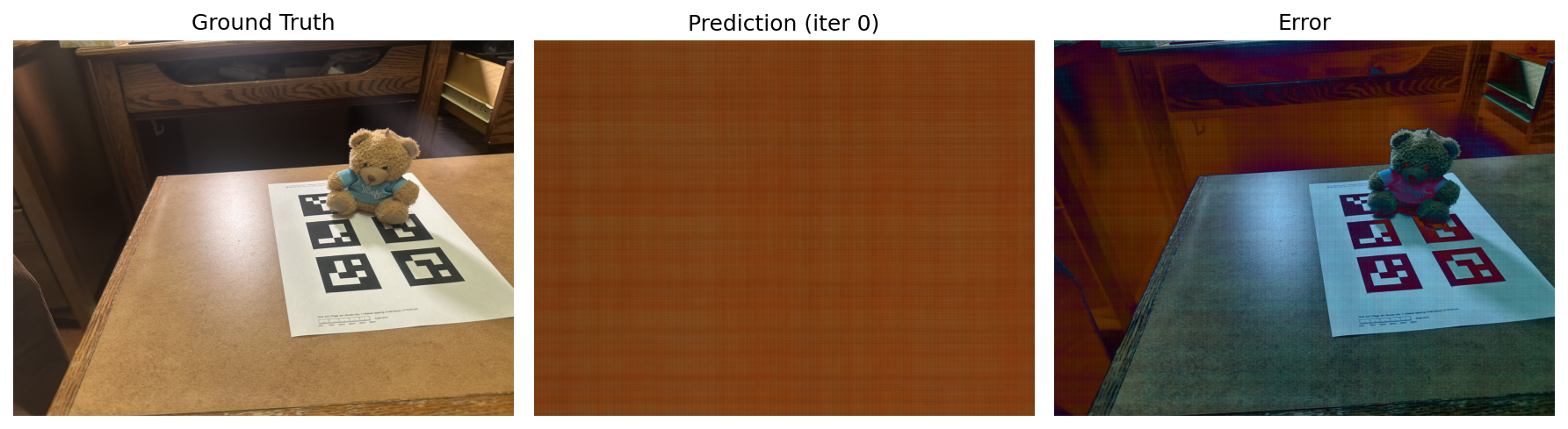
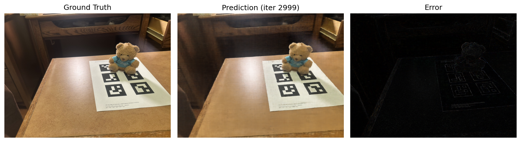
The following grids show how the neural field sharpens each image across training iterations.
Test Image (Fox)
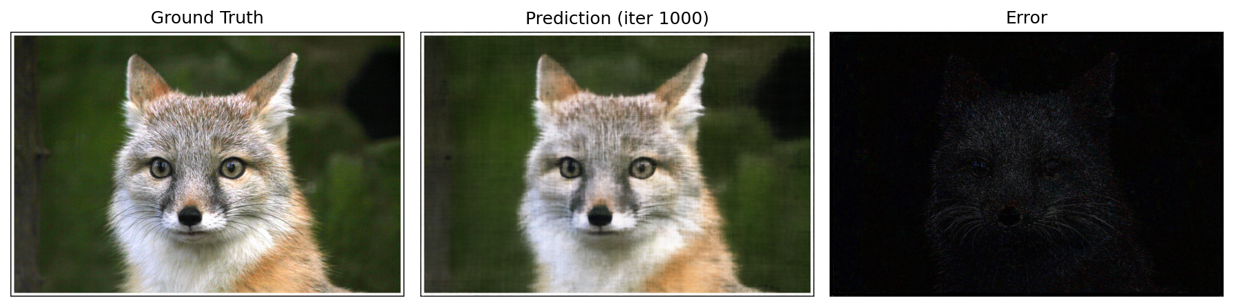
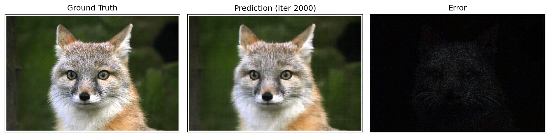
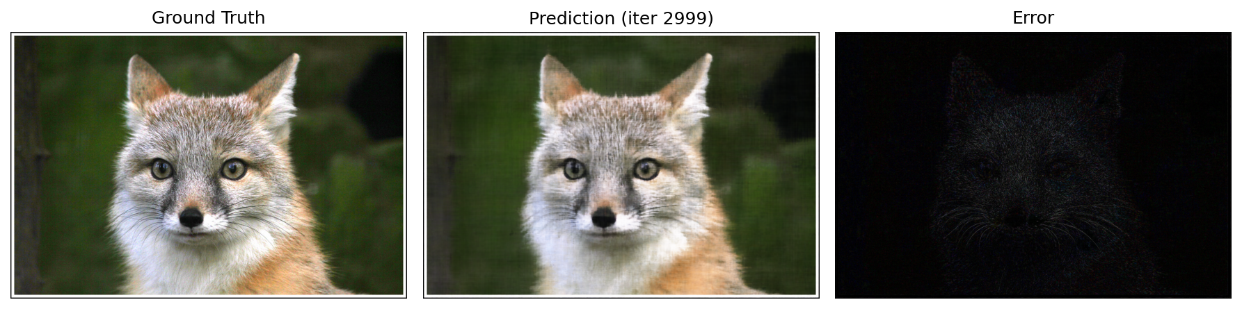
My Own Image (CalHacks Bear)
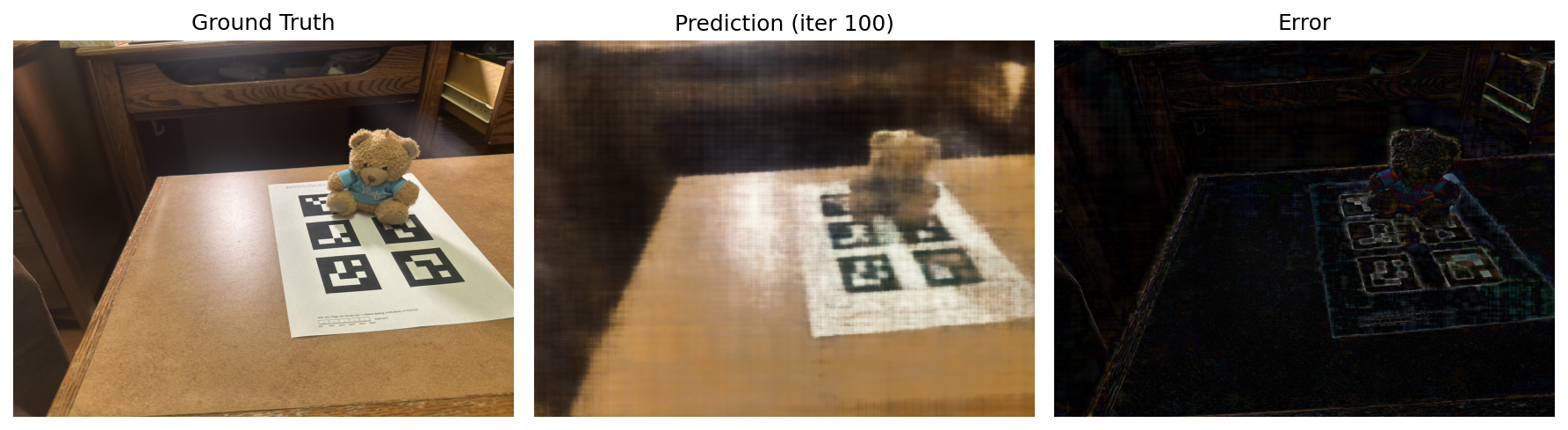
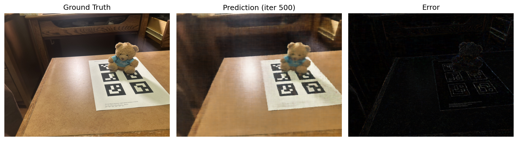
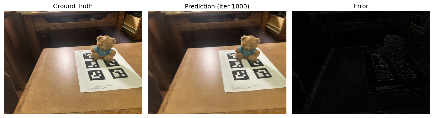
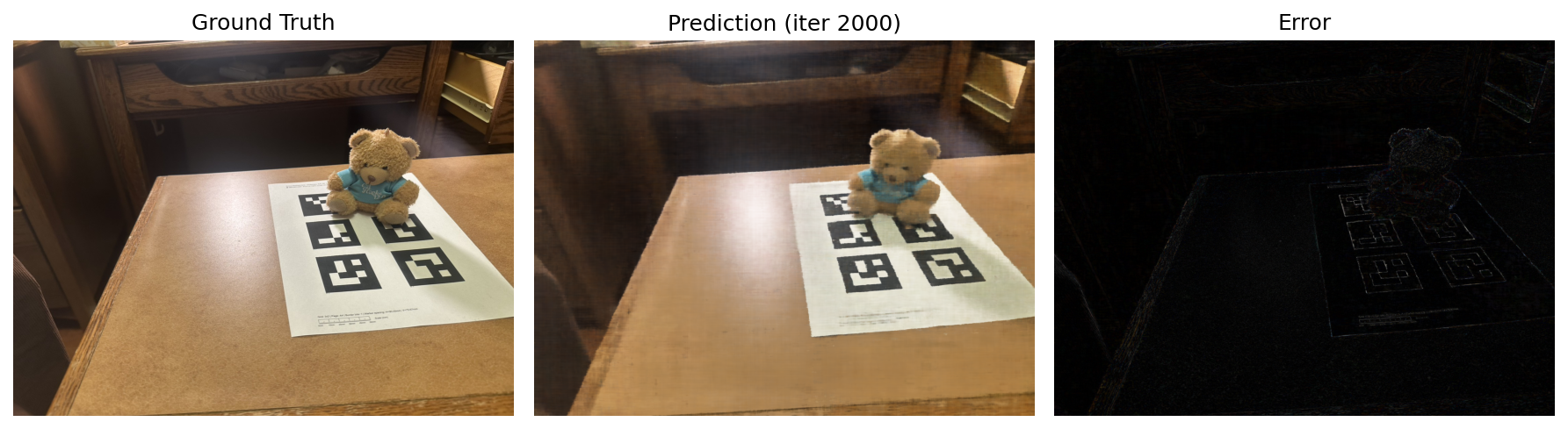
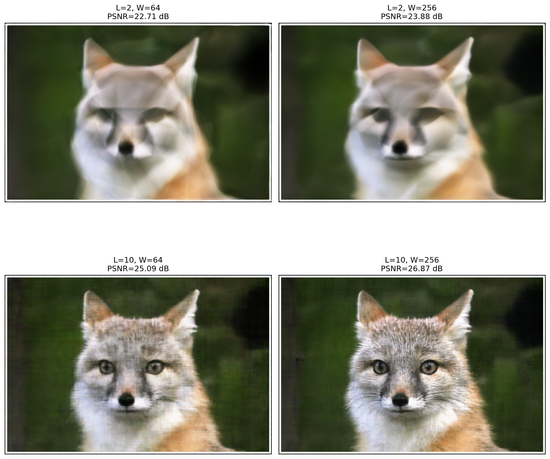
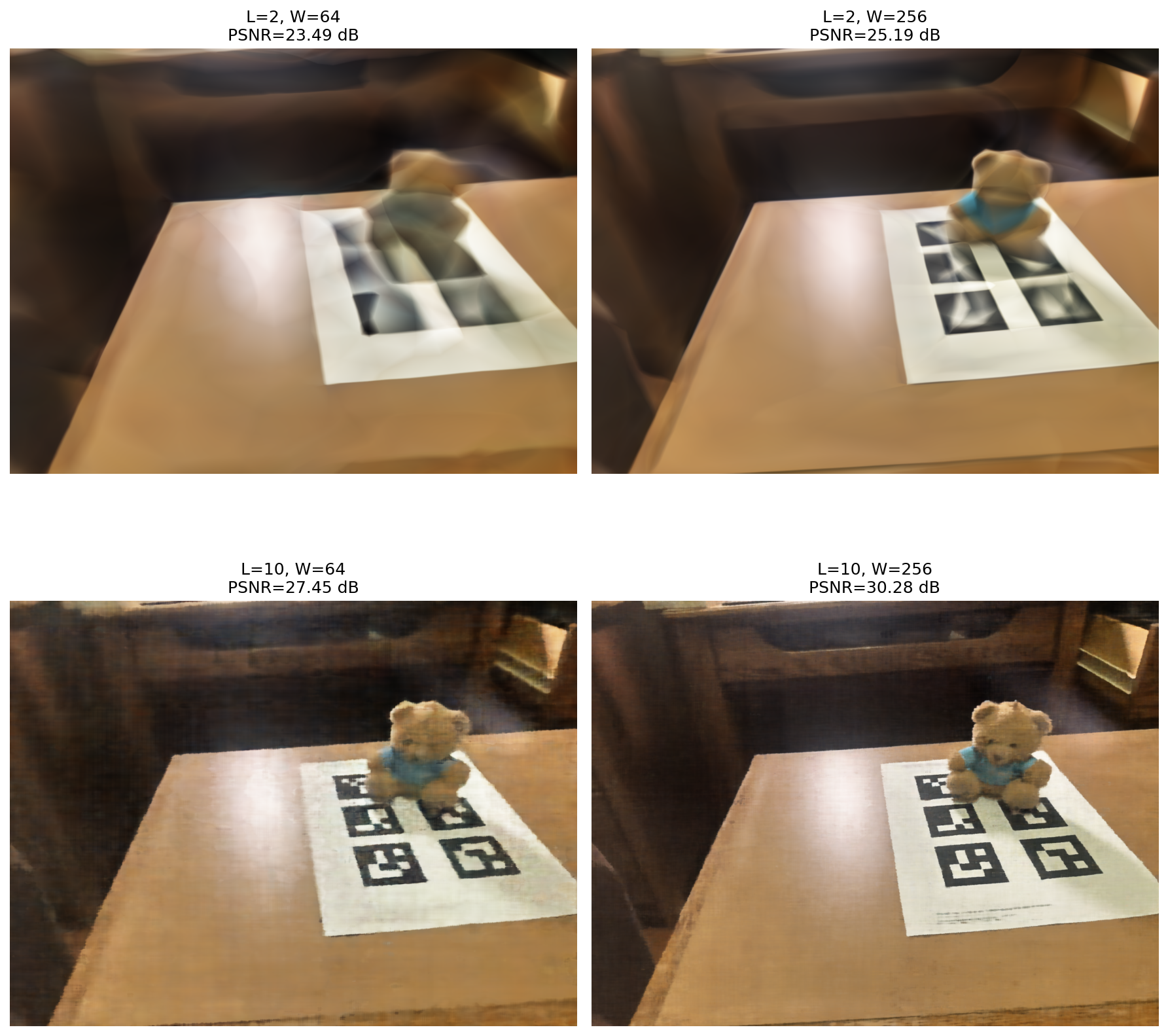
3) Hyperparameter Tuning
We experiment with different values of L and layer width to understand their impact on reconstruction quality.
Using very low values reveals how these hyperparameters affect the model's ability to capture fine details.
Observations
- Positional Encoding (L): Lower L values struggle to capture high-frequency details, resulting in blurry outputs. Higher L values enable the network to represent fine textures and edges.
- Layer Width: Narrower networks (fewer neurons per layer) have limited capacity, leading to smoother, less detailed reconstructions. Wider networks can fit more complex patterns.
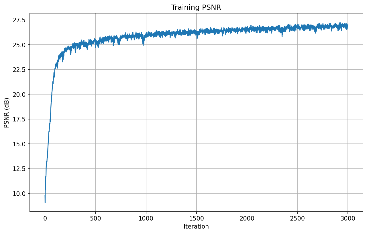
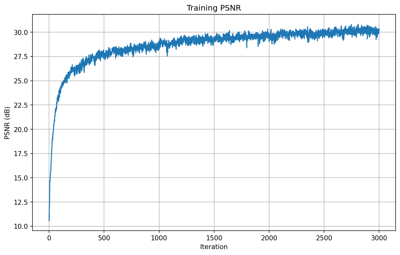
4) Training PSNR Curves
This shows reconstruction quality improvement during training. Higher PSNR indicates better image quality.
The __main__ block above performs a quick sanity sweep: verifying UV indexing, sampling random rays, and ensuring sample_along_rays still produces reasonable shapes before plugging the dataloader into training.
Part 2.1: Ray Generation
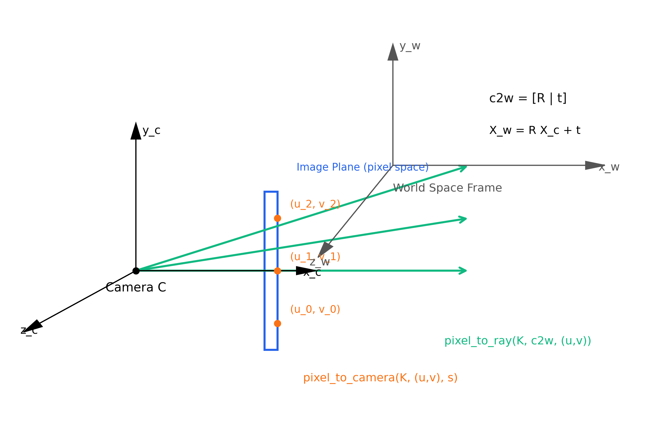
This step turns every 2D pixel into a 3D ray—that’s the data the NeRF will actually learn from. For each pixel we recover its camera-space direction, rotate/translate it into world space using the pose, and treat the camera center plus that direction as a ray ready for sampling.
Coordinate Conventions
- Intrinsic matrix K: Encodes the focal lengths
f_x, f_yand principal point(o_x, o_y). I assume square pixels sof_x = f_y = focalwhen using the provided synthetic datasets. - Extrinsics: I store poses as camera-to-world (c2w) matrices, which is the inverse of OpenCV’s w2c output. Each pose is
[R | t]wheretis the camera origin expressed in world space. - Pixel centers: Following the spec, I add
0.5to each integer pixel index so that rays pass through pixel centers when forming the meshgrid.
Implementation
The code mirrors the three conceptual blocks above. First, pixel_to_camera undoes the projection equation s · [u, v, 1]^⊤ = K · [x_c, y_c, z_c]^⊤. Then pixel_to_ray rotates and translates those points into world space and subtracts the camera origin to obtain directions. Finally, get_rays packages everything for a full-resolution image by creating a dense grid of pixel centers.
Ray Generation Functions (PyTorch)
def pixel_to_camera(K, uv, s, device='cpu'):
    if not isinstance(K, torch.Tensor):
        K = torch.FloatTensor(K).to(device)
    if not isinstance(uv, torch.Tensor):
        uv = torch.FloatTensor(uv).to(device)

    u, v = uv[:, 0], uv[:, 1]
    f_x, f_y = K[0, 0], K[1, 1]
    o_x, o_y = K[0, 2], K[1, 2]

    x_c = (u - o_x) / f_x * s
    y_c = (v - o_y) / f_y * s
    z_c = torch.ones_like(u) * s
    return torch.stack([x_c, y_c, z_c], dim=-1)

def pixel_to_ray(K, c2w, uv):
    if not isinstance(c2w, torch.Tensor):
        c2w = torch.tensor(c2w, dtype=torch.float32)

    device = c2w.device
    x_c = pixel_to_camera(K, uv, s=1.0, device=device)
    R, t = c2w[:3, :3], c2w[:3, 3]

    x_w = (R @ x_c.T).T + t.unsqueeze(0)
    r_o = t.unsqueeze(0).expand_as(x_w)
    r_d = x_w - r_o
    r_d = r_d / torch.norm(r_d, dim=-1, keepdim=True)
    return r_o, r_d

def get_rays(H, W, focal, c2w):
    device = c2w.device if isinstance(c2w, torch.Tensor) else 'cpu'
    K = torch.FloatTensor([
        [focal, 0, W / 2],
        [0, focal, H / 2],
        [0, 0, 1]
    ]).to(device)

    i, j = torch.meshgrid(
        torch.arange(H, device=device),
        torch.arange(W, device=device),
        indexing='ij'
    )
    uv = torch.stack([j + 0.5, i + 0.5], dim=-1).reshape(-1, 2).float()
    return pixel_to_ray(K, c2w, uv)
Part 2.2: Point Sampling
Now that every pixel is a ray, we have to choose a subset of rays per batch and discretize each ray into 3D samples for the NeRF.
Sampling Rays Across Images
I reuse the Part 1 pixel sampler but extend it across all views: pick M images, draw N/M pixels from each, and convert them to rays. Adding +0.5 keeps rays centered on the pixels.
n_rays = 1024
select_inds = np.random.choice(len(rays_o), size=n_rays, replace=False)
rays_o = rays_o[select_inds]
rays_d = rays_d[select_inds]

pts, z_vals = sample_along_rays(rays_o, rays_d, n_samples=64)

print(f'Points shape: {pts.shape}')
print(f'Z values shape: {z_vals.shape}')
print(f'Z values range: [{z_vals.min():.2f}, {z_vals.max():.2f}]')
print(f'First point: {pts[0, 0]}')
Sampling Points Along Rays
Each ray is continuous, so I slice it into n_samples depths between near=2.0 and far=6.0. During training I jitter inside each interval (stratified sampling) so the network doesn’t overfit to a single lattice.
Stratified Sampling Along Rays
def sample_along_rays(rays_o, rays_d, near=2.0, far=6.0,
                      n_samples=64, perturb=True):
    N = rays_o.shape[0]

    # Linear samples in normalized depth, then map to [near, far]
    t_vals = torch.linspace(0., 1., n_samples, device=rays_o.device)
    z_vals = near * (1. - t_vals) + far * t_vals          # (n_samples,)
    z_vals = z_vals.expand(N, n_samples)                  # (N, n_samples)

    if perturb:
        mids = 0.5 * (z_vals[:, :-1] + z_vals[:, 1:])
        upper = torch.cat([mids, z_vals[:, -1:]], dim=-1)
        lower = torch.cat([z_vals[:, :1], mids], dim=-1)
        t_rand = torch.rand_like(z_vals)
        z_vals = lower + (upper - lower) * t_rand

    pts = rays_o.unsqueeze(1) + rays_d.unsqueeze(1) * z_vals.unsqueeze(2)
    return pts, z_vals
The function returns both the sampled 3D coordinates and their depths. Later, the renderer uses z_vals to compute alpha weights and volume accumulation. I typically choose n_samples = 64 for training and disable perturbation at evaluation time for deterministic renders.
Part 2.3: Data Loading
This section is basically Part 1’s pixel sampler leveled up: now every batch needs to return ray origins, ray directions, and the associated RGB colors across all camera views.
Multiview Rays Dataloader
I precompute the rays for each image once, flatten everything, and then sample by indexing into those big tensors. This keeps the per-iteration cost tiny and makes it easy to sanity check correspondence between UV coordinates and RGB values.
RaysData + NerfDataloader (high level)
import torch
import numpy as np
from nerf_part2_1_rays import get_rays

class RaysData:
    def __init__(self, images, K, c2ws, device='cpu'):
        if not isinstance(images, torch.Tensor):
            images = torch.FloatTensor(images)
        if not isinstance(c2ws, torch.Tensor):
            c2ws = torch.FloatTensor(c2ws)

        self.images = images.to(device)
        self.c2ws = c2ws.to(device)
        self.device = device
        N, H, W, _ = self.images.shape

        all_rays_o, all_rays_d, all_pixels, all_uvs = [], [], [], []

        for i in range(N):
            rays_o, rays_d = get_rays(H, W, K, self.c2ws[i])
            all_rays_o.append(rays_o)
            all_rays_d.append(rays_d)
            all_pixels.append(self.images[i].reshape(-1, 3))

            y, x = torch.meshgrid(torch.arange(H, device=device), torch.arange(W, device=device), indexing='ij')
            all_uvs.append(torch.stack([x, y], dim=-1).reshape(-1, 2).long())

        self.rays_o = torch.cat(all_rays_o, dim=0)
        self.rays_d = torch.cat(all_rays_d, dim=0)
        self.pixels = torch.cat(all_pixels, dim=0)
        self.uvs = torch.cat(all_uvs, dim=0)

    def sample_rays(self, n):
        indices = torch.randint(0, len(self.rays_o), (n,), device=self.device)
        return self.rays_o[indices], self.rays_d[indices], self.pixels[indices]

class NeRFDataloader:
    def __init__(self, images, c2ws, K_or_focal, H, W, batch_size, device='cpu'):
        if isinstance(K_or_focal, np.ndarray):
            K = K_or_focal
        else:
            focal = float(K_or_focal)
            K = np.array([[focal, 0, W/2], [0, focal, H/2], [0, 0, 1]])
        self.rays_data = RaysData(images, K, c2ws, device)
        self.batch_size = batch_size

    def sample(self):
        return self.rays_data.sample_rays(self.batch_size)
Validation
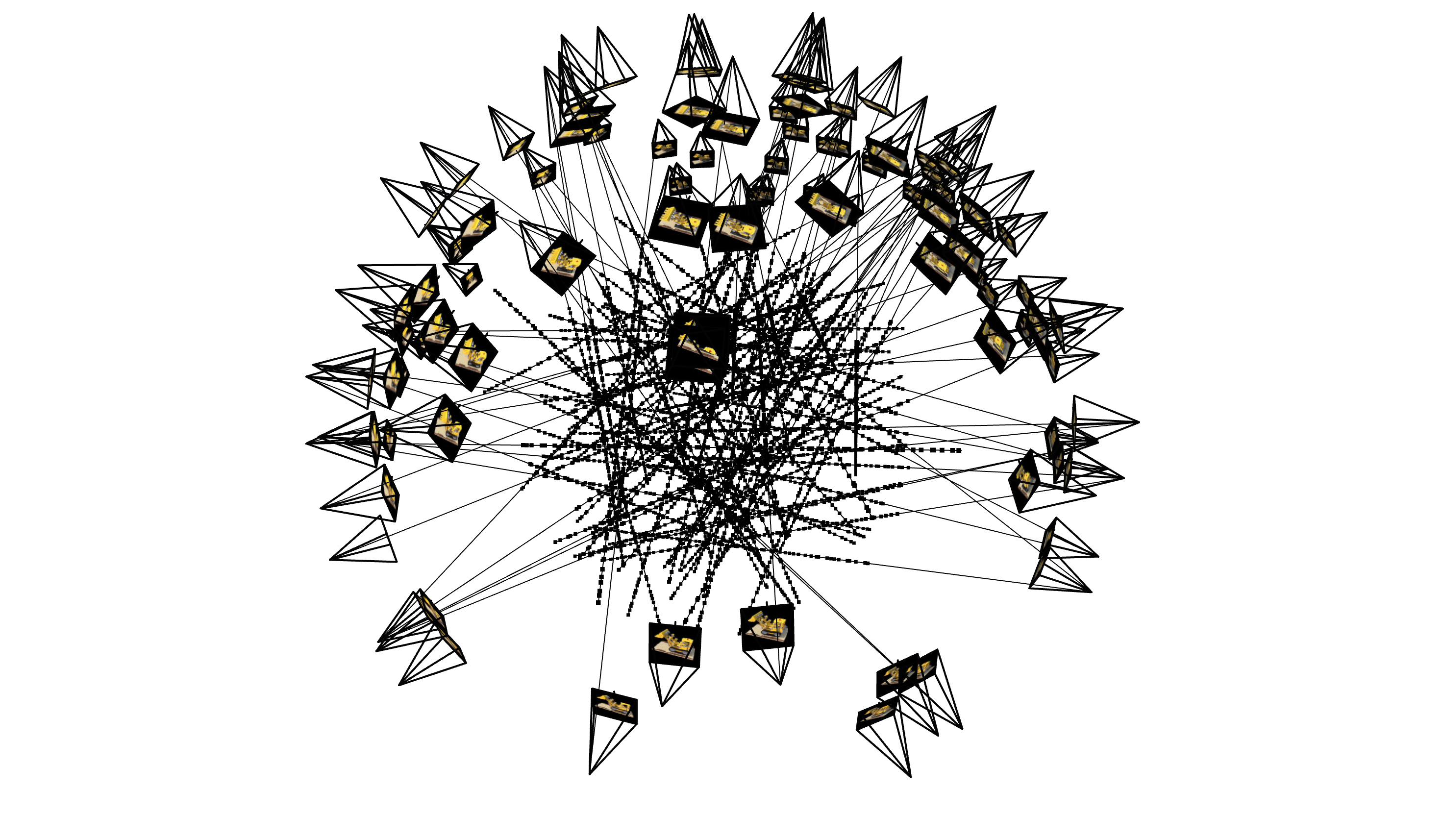
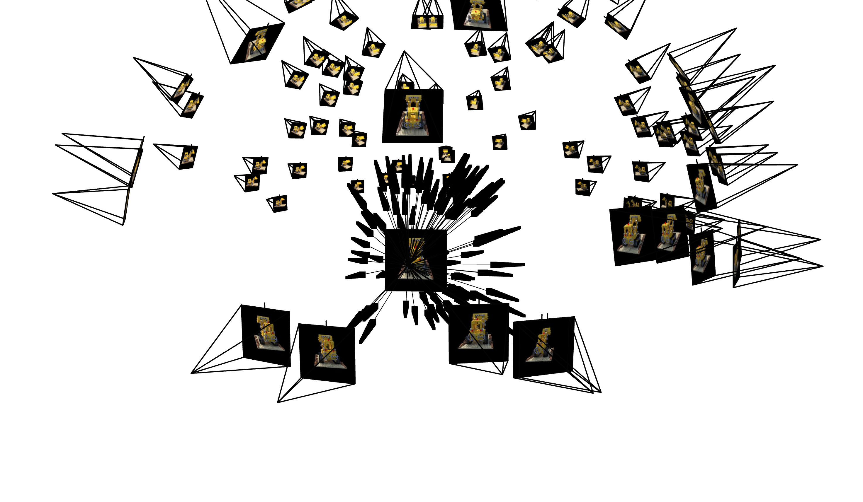
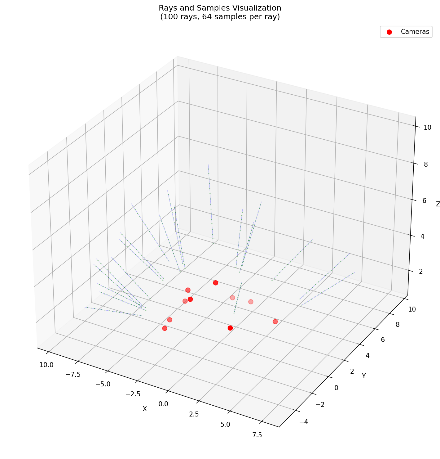
I used the provided plotter to draw camera frustums and sampled rays. Sampling across all views produces a spiky hedgehog, while sampling from a single pose keeps the rays nicely inside one frustum—perfect for catching any indexing bug.
Part 2.4: NeRF Network
The network now needs to map 3D locations and view directions to both color and density. Compared to Part 1’s tiny MLP, this model is deeper, runs on 3D coordinates, and conditions its RGB prediction on the viewing direction.
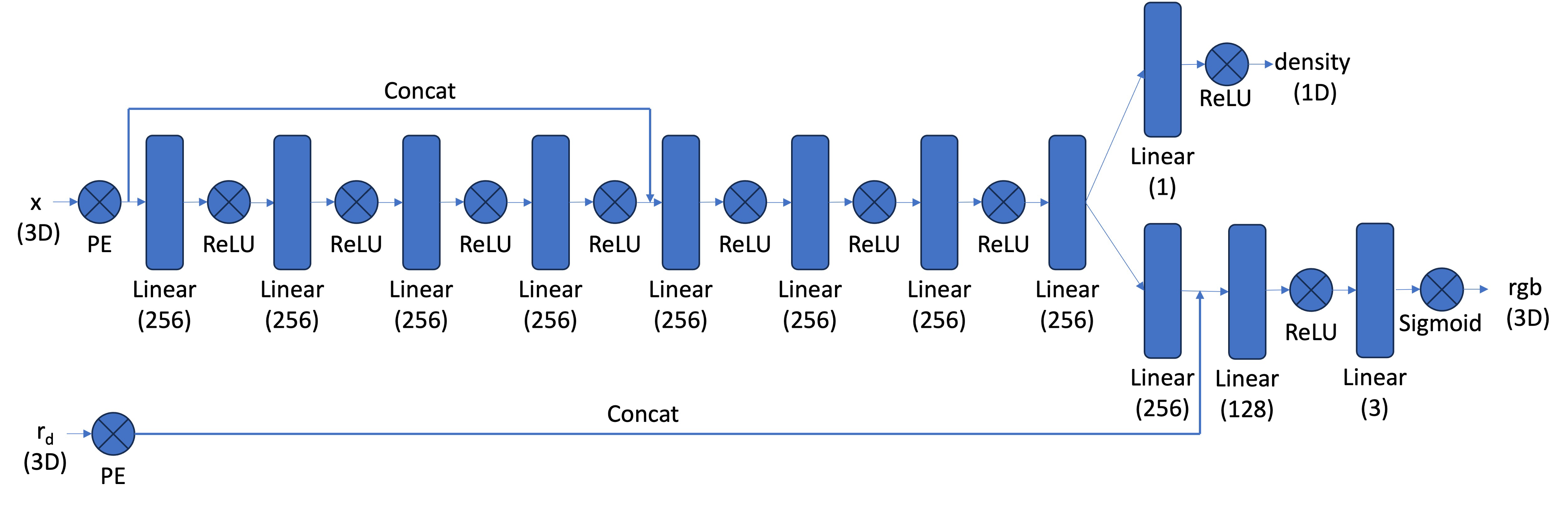
NeRF model (PyTorch)
import torch.nn as nn

class PositionalEncoding(nn.Module):
    def __init__(self, L=10):
        super().__init__()
        self.L = L

    def forward(self, x):
        out = [x]
        for i in range(self.L):
            freq = 2 ** i * np.pi
            out.extend([torch.sin(freq * x), torch.cos(freq * x)])
        return torch.cat(out, dim=-1)

class NeRF(nn.Module):
    def __init__(self, L_pos=10, L_dir=4, hidden_dim=256):
        super().__init__()
        self.pe_pos = PositionalEncoding(L_pos)
        self.pe_dir = PositionalEncoding(L_dir)

        pos_dim = 3 + 3 * 2 * L_pos
        dir_dim = 3 + 3 * 2 * L_dir

        self.lin1 = nn.Linear(pos_dim, hidden_dim)
        self.lin2 = nn.Linear(hidden_dim, hidden_dim)
        self.lin3 = nn.Linear(hidden_dim, hidden_dim)
        self.lin4 = nn.Linear(hidden_dim, hidden_dim)

        self.lin5 = nn.Linear(hidden_dim + pos_dim, hidden_dim)
        self.lin6 = nn.Linear(hidden_dim, hidden_dim)
        self.lin7 = nn.Linear(hidden_dim, hidden_dim)
        self.lin8 = nn.Linear(hidden_dim, hidden_dim)

        self.density_lin = nn.Linear(hidden_dim, 1)
        self.feature_lin = nn.Linear(hidden_dim, hidden_dim)
        self.color_lin1 = nn.Linear(hidden_dim + dir_dim, 128)
        self.color_lin2 = nn.Linear(128, 3)

        nn.init.constant_(self.density_lin.bias, 0.1)

    def forward(self, pts, dirs):
        pts_enc = self.pe_pos(pts)
        dirs_enc = self.pe_dir(dirs)

        x = torch.relu(self.lin1(pts_enc))
        x = torch.relu(self.lin2(x))
        x = torch.relu(self.lin3(x))
        x = torch.relu(self.lin4(x))
        x = torch.cat([x, pts_enc], dim=-1)
        x = torch.relu(self.lin5(x))
        x = torch.relu(self.lin6(x))
        x = torch.relu(self.lin7(x))
        x = torch.relu(self.lin8(x))

        sigma = torch.relu(self.density_lin(x))
        feat = self.feature_lin(x)
        feat_dir = torch.cat([feat, dirs_enc], dim=-1)
        rgb = torch.relu(self.color_lin1(feat_dir))
        rgb = torch.sigmoid(self.color_lin2(rgb))
        return rgb, sigma

model = NeRF(L_pos=10, L_dir=4, hidden_dim=256)
Part 2.5: Volume Rendering
This is where the neural outputs turn into actual pixels. Given densities σ, colors c, and depths z sampled along every ray, we integrate them with the discrete volume-rendering equation from the handout:

Volume rendering helpers
import torch
import numpy as np

def volrend(sigmas, rgbs, step_size):
    N, n_samples = sigmas.shape[:2]
    dists = torch.full((N, n_samples), step_size, device=sigmas.device)
    alpha = 1.0 - torch.exp(-sigmas.squeeze(-1) * dists)
    trans = torch.cumprod(
        torch.cat([torch.ones_like(alpha[:, :1]), 1.0 - alpha[:, :-1]], dim=-1),
        dim=-1
    )
    weights = alpha * trans
    return torch.sum(weights.unsqueeze(-1) * rgbs, dim=1)

def volume_rendering(rgb, sigma, z_vals, rays_d, white_bkgd=False):
    dists = z_vals[:, 1:] - z_vals[:, :-1]
    dists = torch.cat([dists, torch.full_like(dists[:, :1], 1e10)], dim=-1)
    dists = dists * torch.norm(rays_d, dim=-1, keepdim=True)

    alpha = 1.0 - torch.exp(-sigma.squeeze(-1) * dists)
    trans = torch.cumprod(
        torch.cat([torch.ones_like(alpha[:, :1]), 1.0 - alpha[:, :-1]], dim=-1),
        dim=-1
    )
    weights = alpha * trans

    rgb_map = torch.sum(weights.unsqueeze(-1) * rgb, dim=1)
    depth_map = torch.sum(weights * z_vals, dim=-1)
    acc_map = torch.sum(weights, dim=-1)

    if white_bkgd:
        rgb_map = rgb_map + (1.0 - acc_map.unsqueeze(-1))
    return rgb_map, depth_map, acc_map
Run Part 2 on the Lego Dataset
I packaged all subcomponents into a single script that reproduces the NeRF paper’s Lego experiment. It handles argument parsing, ray sampling, training, validation renders, and novel-view generation.
CLI + imports
import os
import sys

if __name__ == '__main__':
    import argparse
    parser = argparse.ArgumentParser()
    parser.add_argument('--dataset', type=str, default='lego',
                        choices=['lego', 'lafufu', 'mydata', 'rabbit', 'miffy', 'all'])
    parser.add_argument('--multi_gpu', action='store_true')
    parser.add_argument('--gpu', type=str, default=None,
                        help='GPU device ID (e.g., "0" or "0,1,2")')
    args = parser.parse_args()

    if args.gpu is not None:
        os.environ['CUDA_VISIBLE_DEVICES'] = args.gpu
        print(f'Using GPU(s): {args.gpu}')
else:
    args = None

import torch
import torch.nn as nn
import numpy as np
import matplotlib.pyplot as plt
from PIL import Image
from tqdm import tqdm

from nerf_part2_1_rays import get_rays
from nerf_part2_2_sampling import sample_along_rays
from nerf_part2_3_dataloader import NeRFDataloader
from nerf_part2_4_network import NeRF
from nerf_part2_5_rendering import volume_renderingRendering helpers
def render_rays(model, rays_o, rays_d, n_samples, near, far,
               device, white_bkgd=True, perturb=False):
    pts, z_vals = sample_along_rays(rays_o, rays_d, near, far,
                                    n_samples, perturb=perturb)

    N, S = pts.shape[:2]
    pts_flat = pts.reshape(-1, 3)
    dirs_flat = rays_d.unsqueeze(1).expand(-1, S, -1).reshape(-1, 3)

    rgb, sigma = model(pts_flat, dirs_flat)
    rgb = rgb.reshape(N, S, 3)
    sigma = sigma.reshape(N, S, 1)

    return volume_rendering(rgb, sigma, z_vals, rays_d,
                            white_bkgd=white_bkgd)

def render_image(model, c2w, H, W, K_or_focal, chunk=1024,
                 n_samples=64, near=2.0, far=6.0, device='cpu',
                 white_bkgd=True):
    rays_o, rays_d = get_rays(H, W, K_or_focal, c2w)
    rays_o, rays_d = rays_o.to(device), rays_d.to(device)

    rgb_chunks = []
    for i in range(0, len(rays_o), chunk):
        rgb, _, _ = render_rays(model,
                                rays_o[i:i+chunk],
                                rays_d[i:i+chunk],
                                n_samples, near, far,
                                device=device, white_bkgd=white_bkgd,
                                perturb=False)
        rgb_chunks.append(rgb.cpu())

    rgb_map = torch.cat(rgb_chunks, dim=0).reshape(H, W, 3)
return rgb_map.numpy()Training + evaluation utilities
def train_nerf(data_path, n_iters, batch_size, lr,
              n_samples, near, far, save_dir,
              multi_gpu=False, white_bkgd=True):
    os.makedirs(save_dir, exist_ok=True)
    device = torch.device('cuda' if torch.cuda.is_available()
                          else 'mps' if torch.backends.mps.is_available()
                          else 'cpu')
    data = np.load(data_path)
    images_train = data['images_train'] / 255.0
    c2ws_train = data['c2ws_train']
    images_val = data['images_val'] / 255.0
    c2ws_val = data['c2ws_val']
    K = data['K'] if 'K' in data else np.array([
        [data['focal'], 0, images_train.shape[2] / 2],
        [0, data['focal'], images_train.shape[1] / 2],
        [0, 0, 1]
    ])
    H, W = images_train.shape[1:3]

    model = NeRF(L_pos=10, L_dir=4, hidden_dim=256)
    if multi_gpu and torch.cuda.device_count() > 1:
        model = nn.DataParallel(model)
    model = model.to(device)

    optimizer = torch.optim.Adam(model.parameters(), lr=lr)
    criterion = nn.MSELoss()
    dataloader = NeRFDataloader(images_train, c2ws_train, K, H, W,
                                batch_size, device)

    psnr_history = []
    save_iters = [0, 100, 500, 1000, 2000, n_iters - 1]
    for it in tqdm(range(n_iters)):
        model.train()
        rays_o, rays_d, target_rgb = dataloader.sample()
        pred_rgb, _, _ = render_rays(model, rays_o, rays_d,
                                     n_samples, near, far,
                                     device=device, white_bkgd=white_bkgd,
                                     perturb=True)
        loss = criterion(pred_rgb, target_rgb)
        optimizer.zero_grad()
        loss.backward()
        optimizer.step()
        psnr = -10 * torch.log10(loss)
        psnr_history.append(psnr.item())

        if it in save_iters:
            eval_model = model.module if hasattr(model, 'module') else model
            eval_model.eval()
            with torch.no_grad():
                val_img = render_image(
                    eval_model,
                    torch.FloatTensor(c2ws_val[0]),
                    H, W, K,
                    n_samples=n_samples,
                    near=near, far=far,
                    device=device
                )
                plt.figure(figsize=(10, 5))
                plt.subplot(1, 2, 1)
                plt.imshow(images_val[0]); plt.title('Ground Truth'); plt.axis('off')
                plt.subplot(1, 2, 2)
                plt.imshow(np.clip(val_img, 0, 1))
                plt.title(f'Predicted (iter {it})'); plt.axis('off')
                plt.tight_layout()
                plt.savefig(f'{save_dir}/val_{it:04d}.png', dpi=150)
                plt.close()

    plt.figure(figsize=(10, 6))
    plt.plot(psnr_history); plt.xlabel('Iteration')
    plt.ylabel('PSNR (dB)'); plt.grid(True)
    plt.savefig(f'{save_dir}/psnr_curve.png', dpi=150); plt.close()

    model_to_save = model.module if hasattr(model, 'module') else model
    torch.save(model_to_save.state_dict(), f'{save_dir}/model.pth')
    return model, psnr_history

def render_validation_views(model, data_path, save_dir,
                            n_samples, near, far, device):
    os.makedirs(save_dir, exist_ok=True)
    data = np.load(data_path)
    images_val = data['images_val'] / 255.0
    c2ws_val = data['c2ws_val']
    K = data['K'] if 'K' in data else np.array([
        [data['focal'], 0, images_val.shape[2] / 2],
        [0, data['focal'], images_val.shape[1] / 2],
        [0, 0, 1]
    ])
    H, W = images_val.shape[1:3]

    eval_model = model.module if hasattr(model, 'module') else model
    eval_model.eval()
    with torch.no_grad():
        for i in range(len(images_val)):
            pred_img = render_image(eval_model,
                                    torch.FloatTensor(c2ws_val[i]),
                                    H, W, K,
                                    n_samples=n_samples,
                                    near=near, far=far,
                                    device=device)
            fig, axes = plt.subplots(1, 3, figsize=(15, 5))
            axes[0].imshow(images_val[i]); axes[0].set_title('GT'); axes[0].axis('off')
            axes[1].imshow(np.clip(pred_img, 0, 1))
            axes[1].set_title('Prediction'); axes[1].axis('off')
            axes[2].imshow(np.abs(images_val[i] - pred_img))
            axes[2].set_title('Error'); axes[2].axis('off')
            plt.tight_layout()
            plt.savefig(f'{save_dir}/val_{i:02d}.png', dpi=150, bbox_inches='tight')
            plt.close()

def run_lego(multi_gpu=False):
    save_dir = 'images/tmp/nerf'
    data_path = 'dataset/lego_200x200.npz'
    model, psnr_history = train_nerf(
        data_path=data_path,
        n_iters=5000,
        batch_size=10000,
        lr=5e-4,
        n_samples=64,
        near=2.0,
        far=6.0,
        save_dir=save_dir,
        multi_gpu=multi_gpu
    )
    device = torch.device('cuda' if torch.cuda.is_available()
                          else 'mps' if torch.backends.mps.is_available()
                          else 'cpu')
    render_validation_views(model, data_path, save_dir,
                            n_samples=64, near=2.0, far=6.0, device=device)
    render_novel_views(model, data_path, num_frames=120,
                       save_path=f'{save_dir}/novel_views.gif',
                       n_samples=64, near=2.0, far=6.0, device=device)
    print(f'Final PSNR: {psnr_history[-1]:.2f} dB')
Results
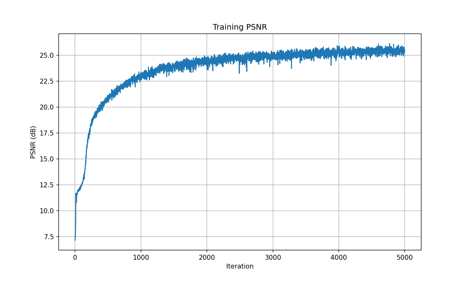
Using the Lego dataset (200×200), I trained with the following settings:
- Iterations: 5,000
- Batch size: 10,000 rays
- Samples per ray: 64 (
near=2.0,far=6.0) - Model: Same NeRF MLP from Part 2.4 with
L_pos=10,L_dir=4 - Optimizer: Adam @
5e-4, white background
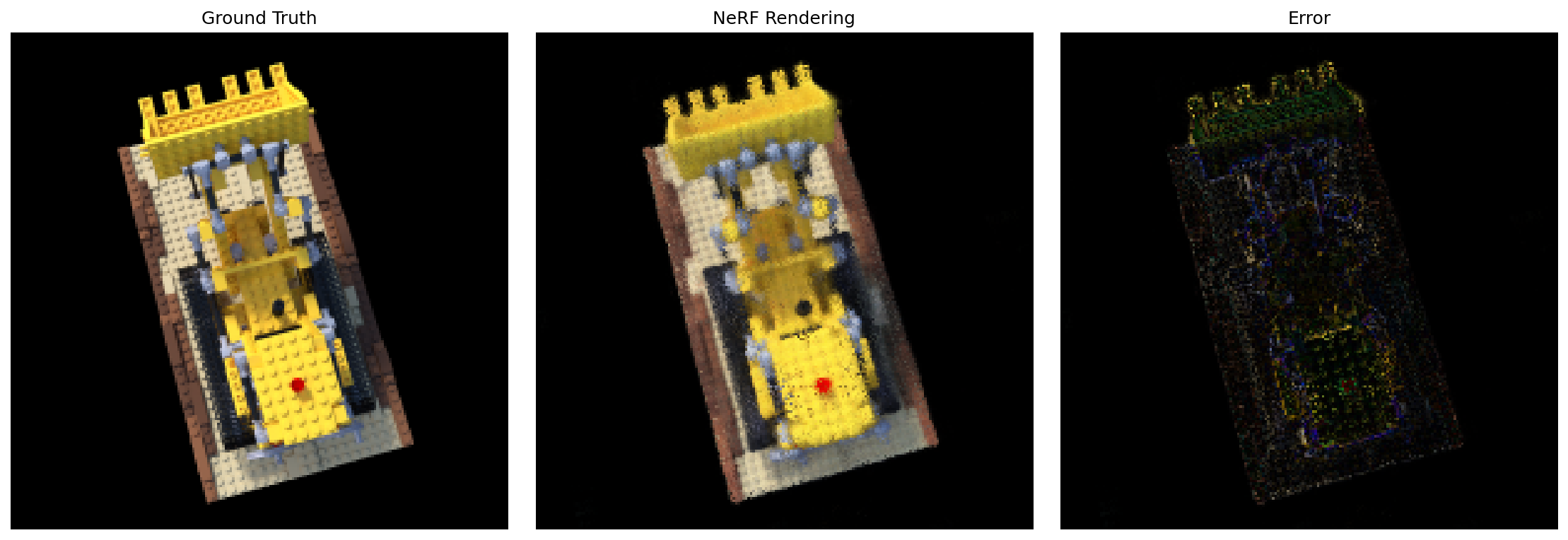
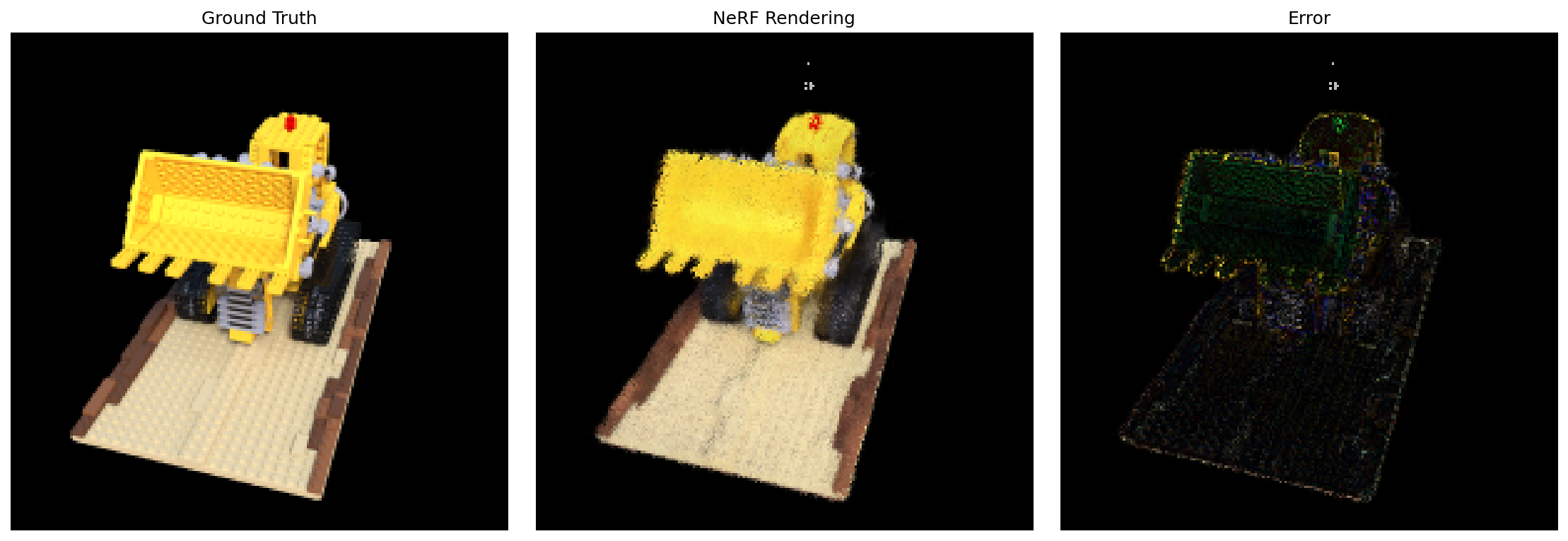
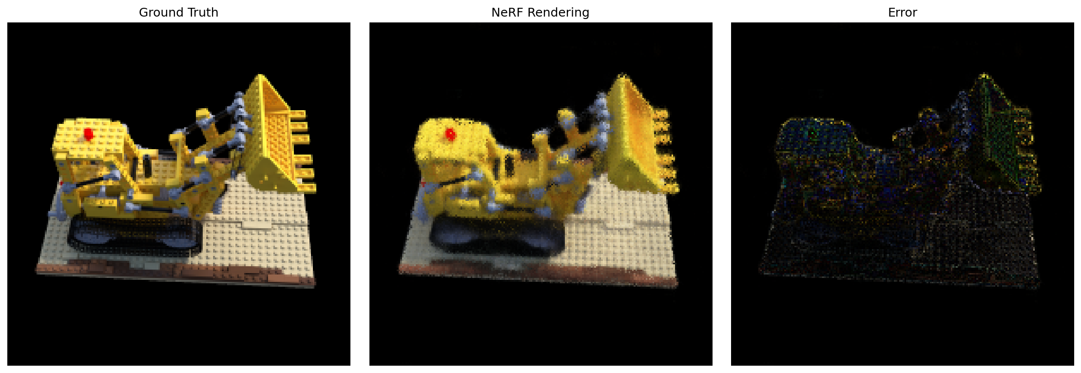
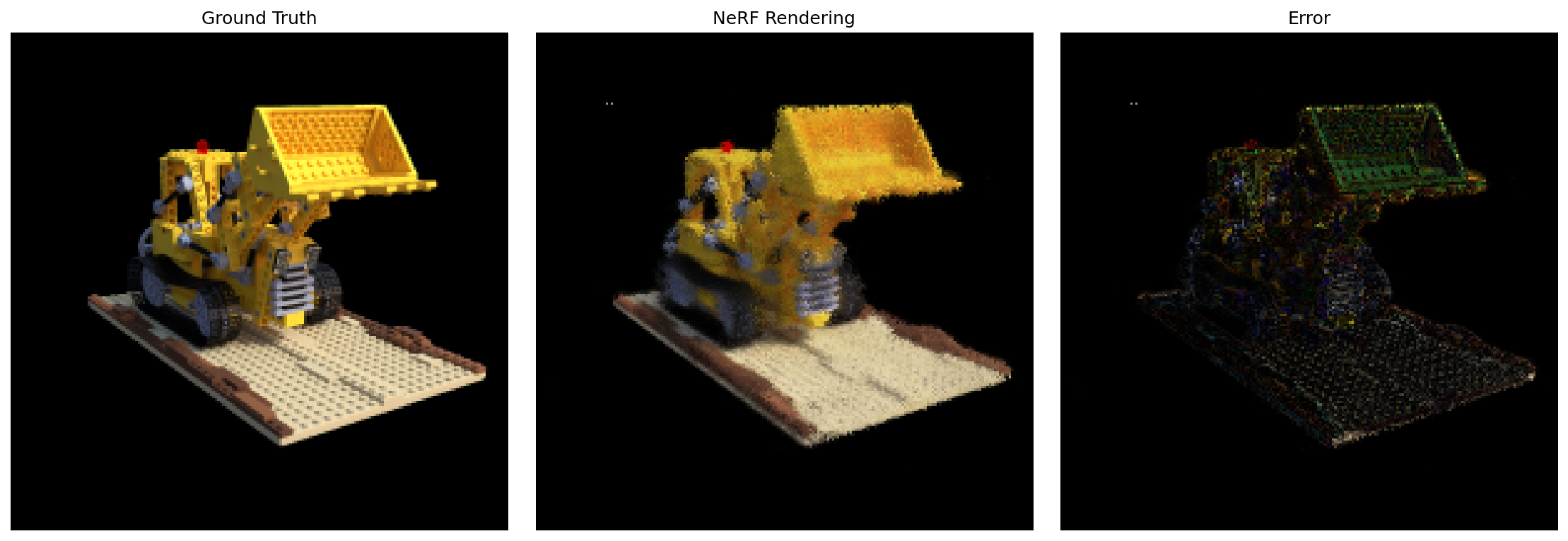
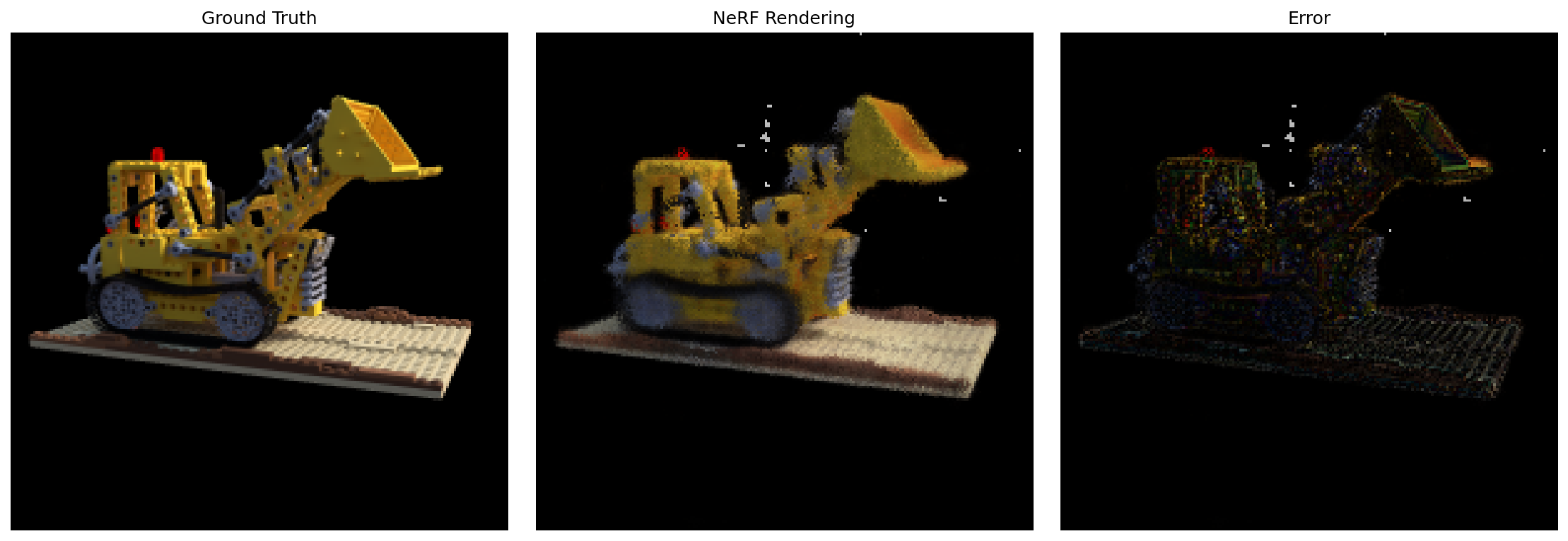
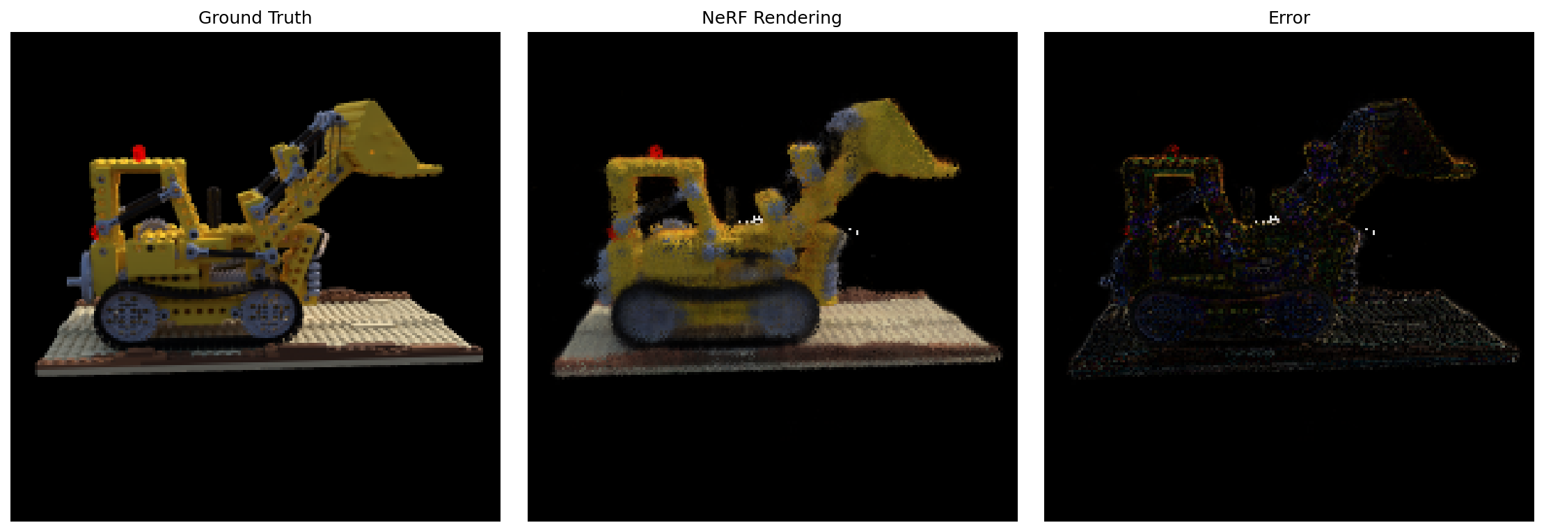
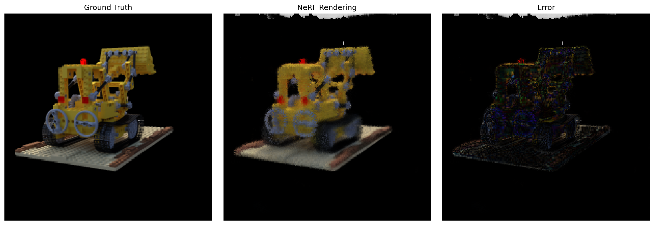
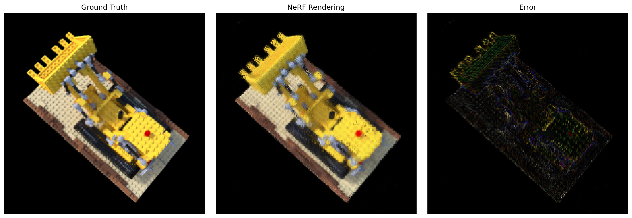
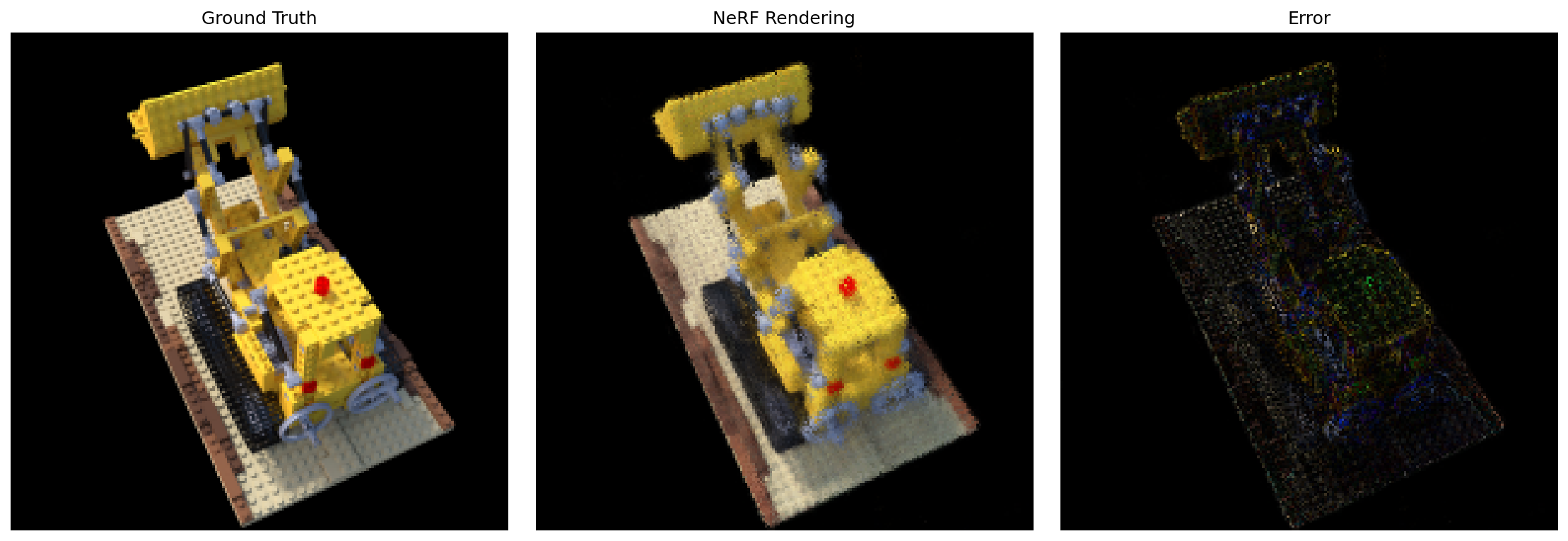
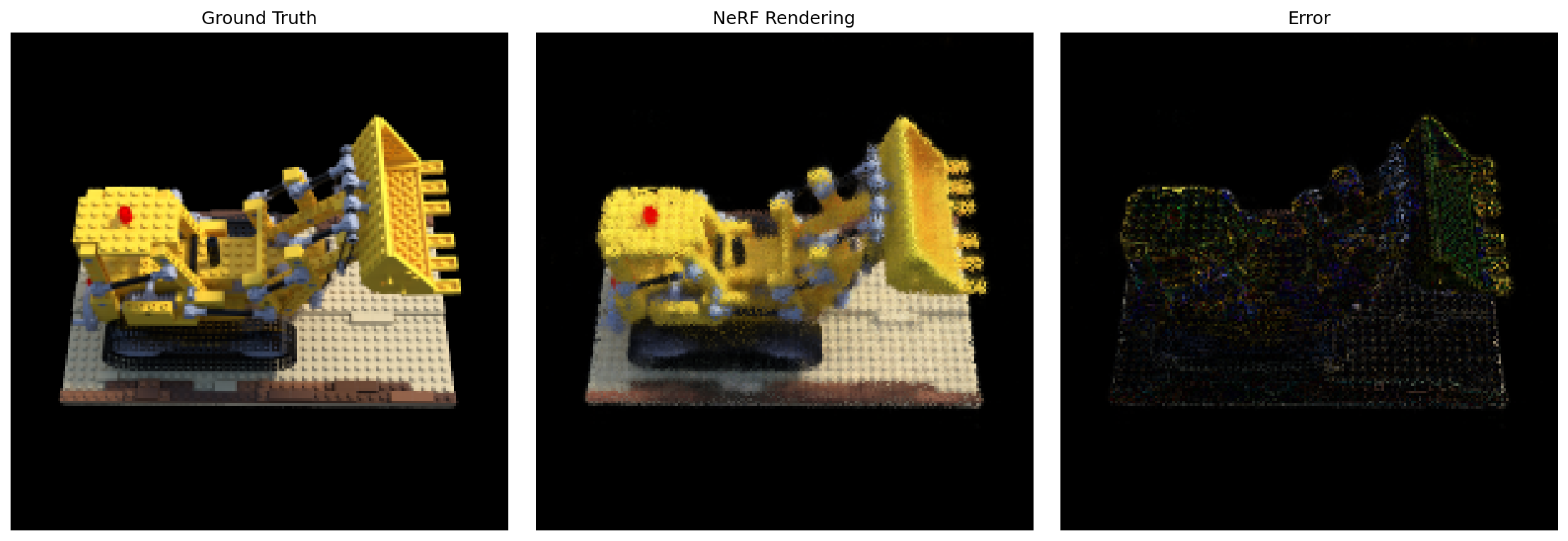
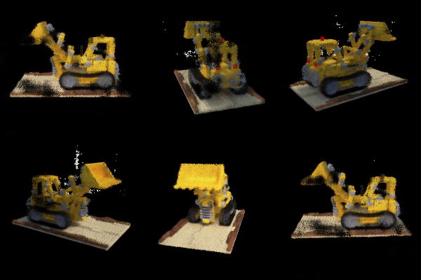
The final model reaches >23 dB PSNR. Below are the intermediate and final visualizations.

Validation set renders:
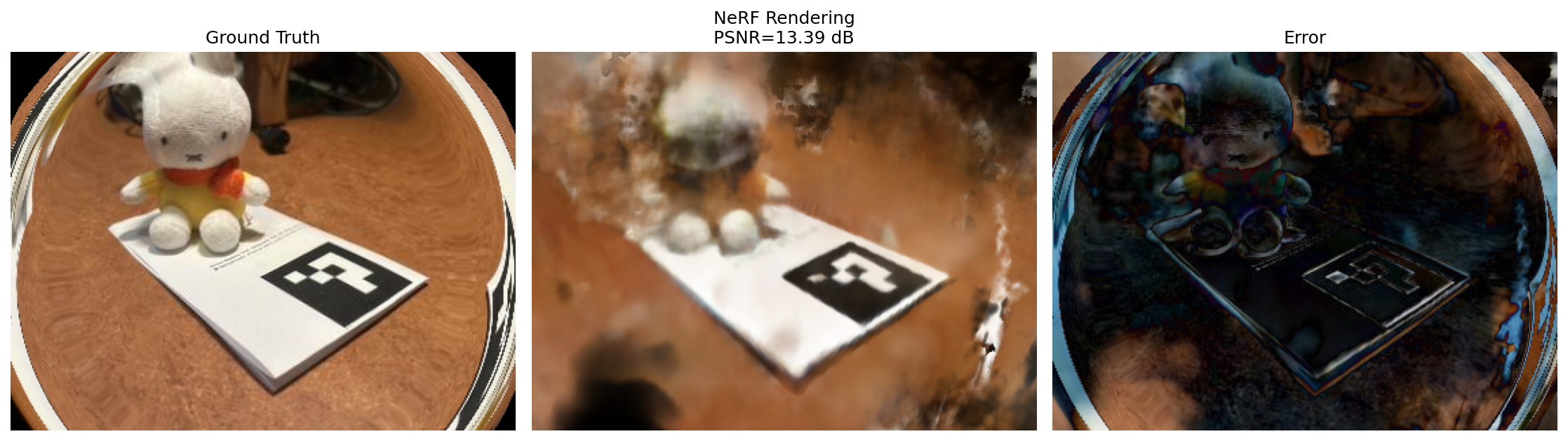
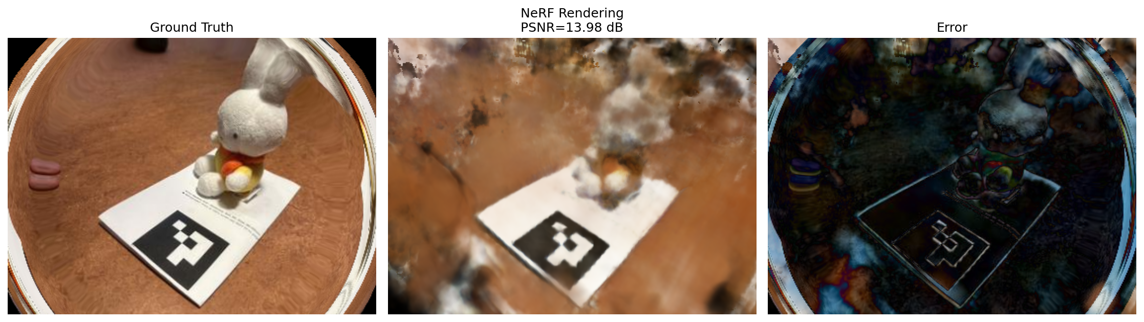
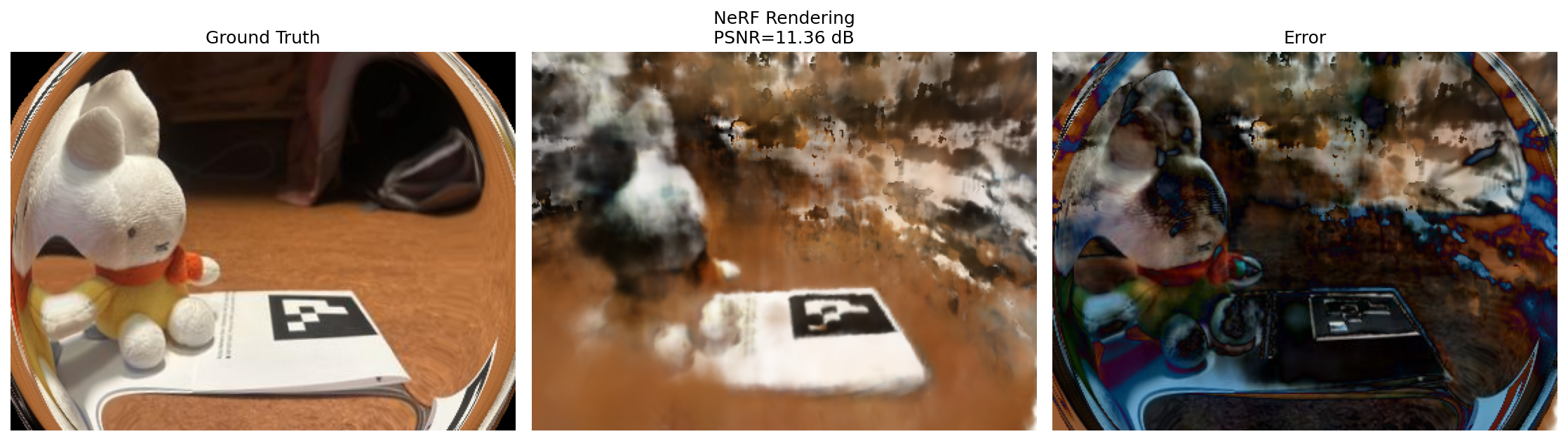
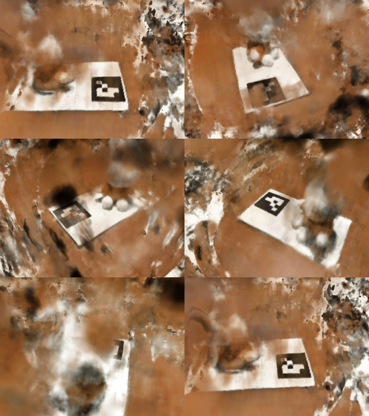
Part 2.6: Training with Custom Data
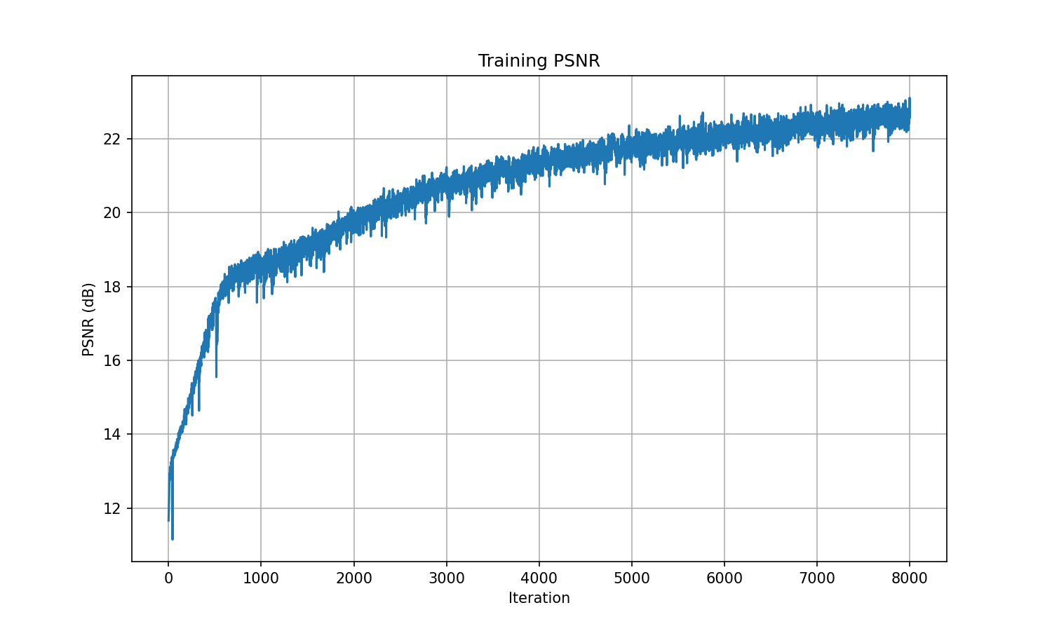
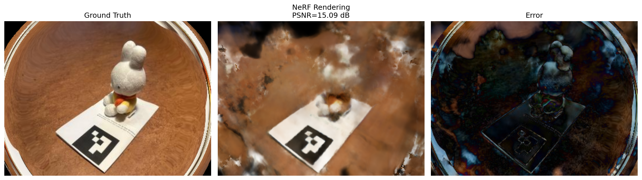
I trained NeRF on my custom Miffy capture. I reused the same model architecture from Part 2.4 (identical NeRF MLP with L_pos=10, L_dir=4) and adjusted the training ranges to match the smaller capture volume.
- Iterations: 8,000
- Batch size: 8,192 rays
- Samples per ray: 128 (
near=0.05,far=0.65) - Optimizer: Adam @
5e-4, white background

Validation set renders:
Debug Notes
I actually shot five different datasets before this run finally converged. The Lafufu set worked from day one, but my captures kept collapsing because the detector latched onto different ArUco IDs in the same sequence. In hindsight the issue was obvious: I taped down a sheet with six tags, so depending on perspective the “active” tag would change mid-frame.

Once I re-shot with a single tag in the scene the pipeline behaved—proof that capture setup matters as much as the NeRF code. (Still not sure why the staff’s Lafufu dataset works with six tags.)
All datasets and trained weights for this whole project are open-sourced here: vaclisinc/2025_Computer_Vision/project_4.